深入GAN学习

注意,实验复现时最好设置随机种子固定Reproducibility — PyTorch 2.0 documentation

1
2
3
4
5
6
7
8
9
10
11
12
13
14

# seed setting
def same_seeds(seed):
    # Python built-in random module
    random.seed(seed)
    # Numpy
    np.random.seed(seed)
    # Torch
    torch.manual_seed(seed)
    if torch.cuda.is_available():
        torch.cuda.manual_seed(seed)
        torch.cuda.manual_seed_all(seed)
    torch.backends.cudnn.benchmark = False
    torch.backends.cudnn.deterministic = True
same_seeds(2023)

GAN

标题Generative Adversarial Nets 2014年

摘要

We propose a new framework for estimating generative models via an adversarial process, in which we simultaneously train two models: a generative model G that captures the data distribution, and a discriminative model D that estimates the probability that a sample came from the training data rather than G. The training procedure for G is to maximize the probability of D making a mistake. This framework corresponds to a minimax two-player game. In the space of arbitrary functions G and D, a unique solution exists, with G recovering the training data distribution and D equal to 1 2 everywhere. In the case where G and D are defined by multilayer perceptrons, the entire system can be trained with backpropagation. There is no need for any Markov chains or unrolled approximate inference networks during either training or generation of samples. Experiments demonstrate the potential of the framework through qualitative and quantitative evaluation of the generated samples

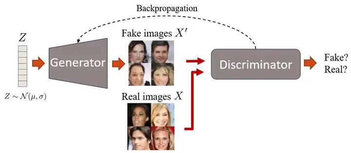
主要贡献:提出GAN 定义G和D以及损失函数.由于GAN中使用的极小极大（minmax）优化，训练可能非常不稳定。

存在问题：梯度不稳定,梯度消失,模式崩溃(特别是NS-GAN,使用了the - log D trick),也就是生成器的损失改为-logD(x)令人拍案叫绝的Wasserstein GAN - 知乎 (zhihu.com)

首先求得生成器固定,最大化V的D

对D(x)求导,让导数为0

将这个最优的D带入一开始的式子

将JS散度带入,有

所以当判别器达到固定G情况下最优时,如果两个分布重叠则为JS则为0,否则JS为log2.梯度一直为0,G得不到更新,所以这种原始GAN会面临梯度消失问题,导致训练困难.

上述的推导都是建立在最优判别器的基础上的，但是在我们实操过程中往往一开始判别器性能是不理想的，所以生成器还是有梯度更新的

如果使用logD-trick,

所以最后需要最小化前面两项,因为后面两项与G无关. 这个最小化目标需要同时最小化KL散度又要最大化JS散度,直观上荒谬,数值结果上导致梯度不稳定,此外第一项的KL散度表示

当P~g~(x)趋近于1,P~r~(x)趋近于0这种情况与当P~g~(x)趋近于0,P~r~(x)趋近于1这种情况对于KL散度情况不一致,由于要最小化KL散度,会导致后者这种情况,也就是

这种情况下,梯度可能不会消失,但会存在梯度不稳定,模式崩溃的问题.

以上内容部分是WGAN中的,从理论上解释了GAN训练的一些问题.

使用tensorboard记录损失

大致流程是首先将损失计入到一个文件,然后使用tensorboard读取,便能使用tensorboard打开一个端口,在网页上查看。torch.utils.tensorboard — PyTorch 2.0 documentation

1
2
3
4
5
6
7
8
9
10
11
12
13
14
15
16
17

!pip install tensorboard
from torch.utils.tensorboard import SummaryWriter 
writer = SummaryWriter('./logs')  

transform = transforms.Compose([transforms.ToTensor(), transforms.Normalize((0.5,), (0.5,))])
trainset = datasets.MNIST('mnist_train', train=True, download=True, transform=transform)
trainloader = torch.utils.data.DataLoader(trainset, batch_size=64, shuffle=True)
model = torchvision.models.resnet50(False)
# Have ResNet model take in grayscale rather than RGB
model.conv1 = torch.nn.Conv2d(1, 64, kernel_size=7, stride=2, padding=3, bias=False)
images, labels = next(iter(trainloader))

grid = torchvision.utils.make_grid(images)
writer.add_image('images', grid, 0)
writer.add_graph(model, images)
# 关闭writer
writer.close()

1
2
3
4
5
6
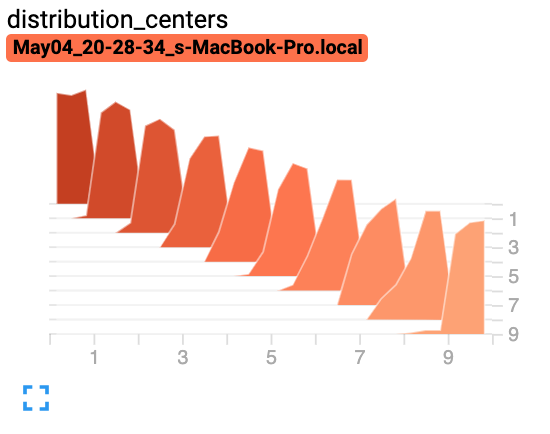
7

from torch.utils.tensorboard import SummaryWriter
import numpy as np
writer = SummaryWriter()
for i in range(10):
    x = np.random.random(1000)
    writer.add_histogram('distribution centers', x + i, i)
writer.close()

在google colab使用需要搭配一些magic func

1
2

%load_ext tensorboard  #使用tensorboard 扩展
%tensorboard --logdir logs  #定位tensorboard读取的文件目录

使用visdom可视化

visdom一般搭配pytorch,毕竟都是meta的.

1
2
3
4
5
6
7
8
9
10
11
12
13
14
15

pip install visdom
python -m visdom.server
iz = Visdom()
  
viz.line([0.],    #Y的第一个点
         [0.],    #X的第一个点
         win="train loss",   #右上角窗口的名称 
         opts=dict(title='train_loss') #opt的参数都可以用python字典的格式传入，还有很多其他的类似matplotlib美化图形的参数参考官网
        )  
        
viz.line([1,],#Y的下一个点
         [1.],#X的下一个点
         win="train loss",
         update='append'#添加到下一个点后面
         )

这里还是推荐选择两者之一即可.

*DCGAN

标题WITH DEEP CONVOLUTIONAL GENERATIVE ADVERSARIAL NETWORKS

intro

Learning reusable feature representations from large unlabeled datasets has been an area of active research. In the context of computer vision, one can leverage the practically unlimited amount of unlabeled images and videos to learn good intermediate representations, which can then be used on a variety of supervised learning tasks such as image classification. We propose that one way to build good image representations is by training Generative Adversarial Networks (GANs) (Goodfellow et al., 2014), and later reusing parts of the generator and discriminator networks as feature extractors for supervised tasks. GANs provide an attractive alternative to maximum likelihood techniques. One can additionally argue that their learning process and the lack of a heuristic cost function (such as pixel-wise independent mean-square error) are attractive to representation learning. GANs have been known to be unstable to train, often resulting in generators that produce nonsensical outputs. There has been very limited published research in trying to understand and visualize what GANs learn, and the intermediate representations of multi-layer GANs. In this paper, we make the following contributions

• We propose and evaluate a set of constraints on the architectural topology of Convolutional GANs that make them stable to train in most settings. We name this class of architectures Deep Convolutional GANs (DCGAN)

• We use the trained discriminators for image classification tasks, showing competitive performance with other unsupervised algorithms.

• We visualize the filters learnt by GANs and empirically show that specific filters have learned to draw specific objects.

We show that the generators have interesting vector arithmetic properties allowing for easy manipulation of many semantic qualities of generated sample

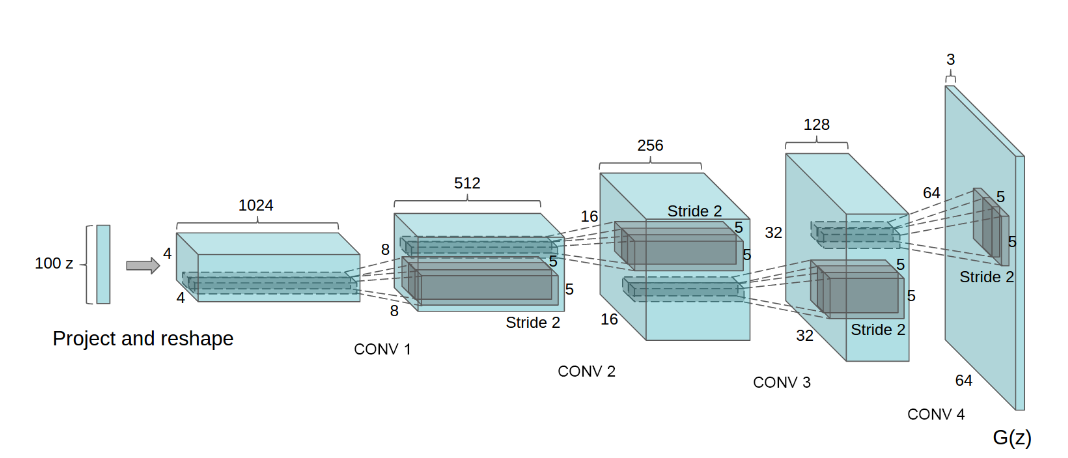
贡献:提出卷积GAN,卷积层替代全连接,使用训练过的判别器用于分类任务,可视化了生成器中的某层,显示出良好的绘制特定对象的能力.生成器的向量显示出能控制样本的语义质量行为.介绍了一些超参的初始化.

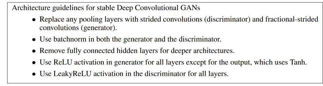
• Replace any pooling layers with strided convolutions (discriminator) and fractional-strided convolutions (generator).

• Use batchnorm in both the generator and the discriminator. • Remove fully connected hidden layers for deeper architectures.

• Use ReLU activation in generator for all layers except for the output, which uses Tanh. • Use LeakyReLU activation in the discriminator for all layers

使用了三个数据集

• 批量标准化是两个网络中必须的。
• 卷积层替代全连接层。
• 使用strided卷积(步幅大于1)可以代替池化
• ReLU激活（几乎总是）会有帮助。

原论文中D判别函数使用的是ReLU,但现在代码中很多其实还是用的LeakyReLU.此外不使用池化,而是使用deconvolution或者叫分数步长卷积(fractionally-strided convolutions).

pytorch实现中,D判别器使用nn.AvgPool2d平均池化操作.

layer normalization RNN,nlp任务中,每个token的特征数不同,针对每个token

instance normalization GAN中,针对单个图像不同的通道

InstanceNorm2d and LayerNorm are very similar, but have some subtle differences. InstanceNorm2d is applied on each channel of channeled data like RGB images, but LayerNorm is usually applied on entire sample and often in NLP tasks. Additionally, LayerNorm applies elementwise affine transform, while InstanceNorm2d usually don’t apply affine transform

ConvTranspose2d

逆卷积fractionally-strided convolutions,可以利用torchsummary这个库查看模型相关信息

1
2

myModel = Discriminator().to(DEVICE)
summary(myModel,(1,28,28))

1
2
3
4
5
6
7
8
9
10
11
12
13
14
15
16
17
18
19
20
21
22
23
24
25

----------------------------------------------------------------
        Layer (type)               Output Shape         Param #
================================================================
            Conv2d-1          [-1, 512, 14, 14]           4,608
       BatchNorm2d-2          [-1, 512, 14, 14]           1,024
         LeakyReLU-3          [-1, 512, 14, 14]               0
            Conv2d-4            [-1, 256, 7, 7]       1,179,648
       BatchNorm2d-5            [-1, 256, 7, 7]             512
         LeakyReLU-6            [-1, 256, 7, 7]               0
            Conv2d-7            [-1, 128, 4, 4]         294,912
       BatchNorm2d-8            [-1, 128, 4, 4]             256
         LeakyReLU-9            [-1, 128, 4, 4]               0
        AvgPool2d-10            [-1, 128, 1, 1]               0
           Linear-11                    [-1, 1]             129
          Sigmoid-12                    [-1, 1]               0
================================================================
Total params: 1,481,089
Trainable params: 1,481,089
Non-trainable params: 0
----------------------------------------------------------------
Input size (MB): 0.00
Forward/backward pass size (MB): 2.63
Params size (MB): 5.65
Estimated Total Size (MB): 8.28
----------------------------------------------------------------

我在测试github上一个DCGAN的代码时,发现其在生成器上除了最后一层使用tanh激活函数,其他层都使用leak激活函数,但是这样生成器会逐渐变大.

因为LeakyReLU照顾到了负数,使得每一线性层输出为负值时也有梯度,这样也许能使得生成器跳出

*WGAN

使用EM距离GAN — Wasserstein GAN & WGAN-GP. Training GAN is hard. Models may never… | by Jonathan Hui | Medium

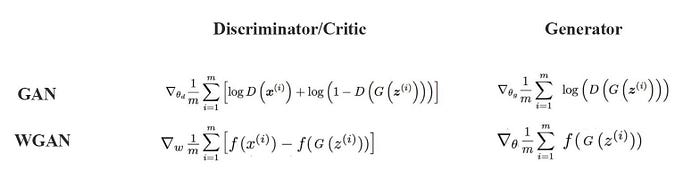
• 判别器最后一层去掉sigmoid
• 生成器和判别器的loss不取log
• 每次更新判别器的参数之后把它们的绝对值截断到不超过一个固定常数c
• 不要用基于动量的优化算法（包括momentum和Adam），推荐RMSProp，SGD也行

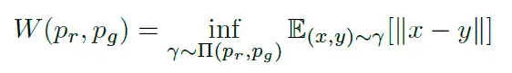
上面这个公式是基于推图距离的计算

下面是WGAN论文的intro

一开始的GAN的损失函数设计被认为有问题,与KL,JS散度有关.

KL散度是熵与交叉熵的差,它不是对称的.

而JS散度和KL散度是有关联的,可以看出JS散度是对称的,

经证明,当两个分布不重叠时,JS散度为log2GAN：两者分布不重合JS散度为log2的数学证明_为什么深度学习wganjs散度等于log2

从理论和经验上来说，真实的数据分布通常是一个低维流形，简单地说就是数据不具备高维特性，而是存在一个嵌入在高维度的低维空间内,在实际操作中，我们的维度空间远远不止3维，有可能是上百维，在这样的情况下，数据就更加难于重合.

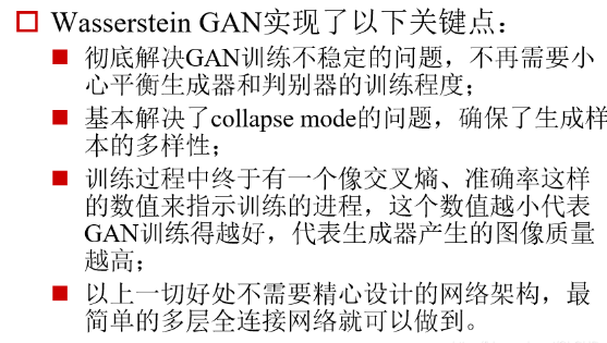
WGAN打算训练网络得到一个函数,这个函数满足1-Lipschitz,同时也是D辨别器,这样能使得损失函数更有意义,也能解决梯度与模式崩溃问题.

WGAN贡献:解决GAN训练不稳定与模式崩溃问题,有一个指标(EM距离),这个值越小训练得越好.

WGAN-GP

这里的GP就是gradient penalty的意思.在发了第一篇GAN的文章之后,作者又发了这篇.

The recently proposed Wasserstein GAN (WGAN) makes progress toward stable training of GANs, but sometimes can still generate only poor samples or fail to converge. We find that these problems are often due to the use of weight clipping in WGAN to enforce a Lipschitz constraint on the critic, which can lead to undesired behavior

WGAN以及其衍生主要都是为了满足Lipschitz constraint,包括后面的Spectral Normalizaton1802.05957.pdf (arxiv.org).

意思是强制使用梯度裁剪(clamp)到一个范围会导致不想要的行为,因为本身想要的是让critic满足Lipschitz,所以粗暴地使用了梯度裁剪.

需要使得判别器f的梯度范数处处小于1,WGAN-GP证明了需要使得在真实数据和生成的数据之间插值的点对于f应该具有1的梯度范数。

范数有多种.

所以需要使用到梯度,而且是对于输入的梯度,通过限制输入的梯度,而不是WGAN中限制每次模型的weight和bias的值.torch.autograd.grad — PyTorch 2.0 documentation在pytorch中使用autograd.grad计算

1
2
3
4
5
6
7
8

import torch
from torch import autograd
# demo
x = torch.rand(3, 4)
x.requires_grad_()
y = torch.sum(x**2)
grads = autograd.grad(outputs=y, inputs=x,create_graph=True)
print(grads)

1
2
3
4
5
6
7
8
9

# Gradient Penalty (e.g. gradients w.r.t x_penalty)
eps = torch.rand(batch_size, 1, 1, 1).to(DEVICE) # x shape: (64, 1, 28, 28)
x_penalty = eps*x + (1-eps)*x_fake
x_penalty = x_penalty.view(x_penalty.size(0), -1)  # n 1 28*28
p_outputs = D(x_penalty, y)  # N,1
xp_grad = autograd.grad(outputs=p_outputs, inputs=x_penalty, grad_outputs=D_labels, # N 1
                        create_graph=True, retain_graph=True, only_inputs=True)
print(xp_grad)
grad_penalty = p_coeff * torch.mean(torch.pow(torch.norm(xp_grad[0], 2, 1) - 1, 2))

对于辨别器,WGAN一般叫做critic,损失函数,而生成器依旧是

1
2
3
4
5
6

# Wasserstein loss
x_outputs = D(x, y)
z_outputs = D(x_fake, y)
D_x_loss = torch.mean(x_outputs)
D_z_loss = torch.mean(z_outputs)
D_loss = D_z_loss - D_x_loss + grad_penalty

此外不使用BN,批次标准化会在同一批次中的样本之间创建相关性。它影响了梯度惩罚的有效性，实验证实了这一点。

一般可以使用Layer Normalization也就是对单个样本进行归一化.

*Conditional GAN

某种程度上里程碑作品,能够控制GAN生成的东西了,通过添加label,也就是condition.

例如在MNIST数据上,增加数字对应的label的one-hot变量,cat到图像数据上.

1
2
3
4
5
6
7
8
9
10
11
12
13
14
15
16
17
18
19
20
21
22
23
24
25
26
27
28
29
30
31
32
33
34
35
36
37

for epoch in range(max_epoch):
    for idx, (images, labels) in enumerate(data_loader):
        # Training Discriminator
        x = images.to(DEVICE)
        y = labels.view(batch_size, 1)
        y = to_onehot(y).to(DEVICE) # condition
        x_outputs = D(x, y)
        D_x_loss = criterion(x_outputs, D_labels)

        z = torch.randn(batch_size, n_noise).to(DEVICE)
        z_outputs = D(G(z, y), y)
        D_z_loss = criterion(z_outputs, D_fakes)
        D_loss = D_x_loss + D_z_loss
        
        D.zero_grad()
        D_loss.backward()
        D_opt.step()
        
        if step % n_critic == 0:
            # Training Generator
            z = torch.randn(batch_size, n_noise).to(DEVICE)
            z_outputs = D(G(z, y), y)
            G_loss = criterion(z_outputs, D_labels)

            G.zero_grad()
            G_loss.backward()
            G_opt.step()
        
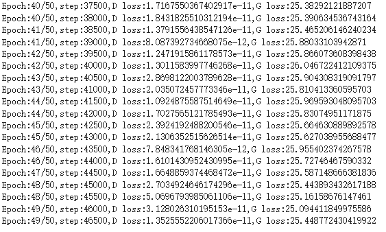
        if step % 500 == 0:
            print('Epoch: {}/{}, Step: {}, D Loss: {}, G Loss: {}'.format(epoch, max_epoch, step, D_loss.item(), G_loss.item()))
        
        if step % 1000 == 0:
            G.eval()
            img = get_sample_image(G, n_noise)
            imsave('samples/{}_step{}.jpg'.format(MODEL_NAME, str(step).zfill(3)), img, cmap='gray')
            G.train()
        step += 1

1
2
3
4
5
6
7
8
9
10
11
12
13
14
15
16
17
18
19
20
21
22
23
24
25
26
27
28
29
30
31
32
33
34
35
36
37
38
39
40
41
42
43
44
45
46
47
48

class Generator(nn.Module):
    """
        Simple Generator w/ MLP
    """
    def __init__(self, input_size=100, condition_size=10, num_classes=784):
        super(Generator, self).__init__()
        self.layer = nn.Sequential(
            nn.Linear(input_size+condition_size, 128),
            nn.LeakyReLU(0.2),
            nn.Linear(128, 256),
            nn.BatchNorm1d(256),
            nn.LeakyReLU(0.2),
            nn.Linear(256, 512),
            nn.BatchNorm1d(512),
            nn.LeakyReLU(0.2),
            nn.Linear(512, 1024),
            nn.BatchNorm1d(1024),
            nn.LeakyReLU(0.2),
            nn.Linear(1024, num_classes),
            nn.Tanh()
        )
        
    def forward(self, x, c):
        x, c = x.view(x.size(0), -1), c.view(c.size(0), -1).float()
        v = torch.cat((x, c), 1) # v: [input, label] concatenated vector
        y_ = self.layer(v)
        y_ = y_.view(x.size(0), 1, 28, 28)
        return y_
class Discriminator(nn.Module):
    """
        Simple Discriminator w/ MLP
    """
    def __init__(self, input_size=784, condition_size=10, num_classes=1):
        super(Discriminator, self).__init__()
        self.layer = nn.Sequential(
            nn.Linear(input_size+condition_size, 512),
            nn.LeakyReLU(0.2),
            nn.Linear(512, 256),
            nn.LeakyReLU(0.2),
            nn.Linear(256, num_classes),
            nn.Sigmoid(),
        )
    
    def forward(self, x, c):        
        x, c = x.view(x.size(0), -1), c.view(c.size(0), -1).float()
        v = torch.cat((x, c), 1) # v: [input, label] concatenated vector
        y_ = self.layer(v)
        return y_

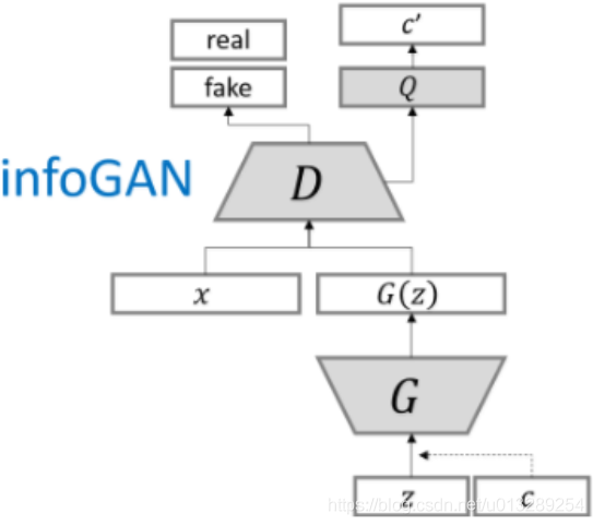
InfoGAN

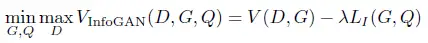
提出利用互信息诱导潜变量.该方法将信息最大化引入到标准GAN网络中。

InfoGAN: Interpretable Representation Learning to Distangle Data Unsupervised | by Renee LIN | MLearning.ai | Medium

期望有良好的特征解耦关系.

GAN公式使用简单的连续输入噪声矢量z，同时对G使用噪声的方式没有限制。因此，噪声可能会被生成器以高度纠缠(entangled)的方式使用，导致 z 的各个维度与数据的语义特征不对应。

在本文中，将输入噪声向量分解为两部分，而不是使用单个非结构化噪声向量：（i）z，它被视为不可压缩噪声源;（ii） c，我们称之为潜在代码，将针对数据分布的显著结构化语义特征。

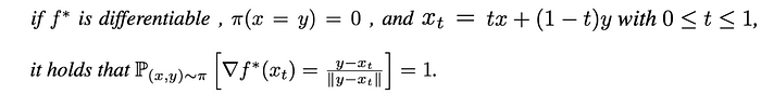
引入互信息,在G输入时加入一个潜变量c,潜在代码 C 和生成器分布 G(z,c) 之间应该有高度的互信息。因此I(c;G(z,c)) 应该很高。给定任何 x ∼ P~G~(x),希望 P~G~（c|x） 有一个较小的熵。换句话说，潜在代码c中的信息不应该在生成过程中丢失。

然而上面互信息的计算涉及后验概率分布P(c|x)，而后者在实际中是很难获取的，所以需要定义一个辅助性的概率分布Q(c|x)，采用Variational Information Maximization对互信息进行下界拟合.

这样互信息计算就能确定最小值,继续推导有

最后目标函数为

z,c均为采样得到,z依旧是正态分布采样,c由两部分组成,一部分是离散分布另一部分是连续分布.论文中使用Categorical与Unif分布,是离散均匀分布与连续均匀分布.

在MNIST数据集上,比如使用c~1~作为离散变量控制生成的数字的类型,其他的c~2~和c~3~作为连续变量控制其他.

1
2
3
4
5
6
7
8
9
10
11
12

def sample_noise(batch_size, n_noise, n_c_discrete, n_c_continuous, label=None, supervised=False):
    z = torch.randn(batch_size, n_noise).to(DEVICE) #正态分布 潜变量 与VAE的中间变量类似. bottleneck
    # 离散分布 控制数字类型也就是类别 如果supervised 会根据label的值
    if supervised:
        c_discrete = to_onehot(label).to(DEVICE) # (B,10)
    else:
        # 否则随机离散均匀生成
        c_discrete = to_onehot(torch.LongTensor(batch_size, 1).random_(0, n_c_discrete)).to(DEVICE) # (B,10)
    # 连续分布 控制其他属性 
    c_continuous = torch.zeros(batch_size, n_c_continuous).uniform_(-1, 1).to(DEVICE) # (B,2)
    c = torch.cat((c_discrete.float(), c_continuous), 1) #c (B,12)
    return z, c

1
2
3
4
5
6
7
8
9
10
11
12
13

 # Training Discriminator
x = images.to(DEVICE)
x_outputs, _, = D(x)
D_x_loss = bce_loss(x_outputs, D_labels)

z, c = sample_noise(batch_size, n_noise, n_c_discrete, n_c_continuous, label=labels, supervised=True)
z_outputs, _, = D(G(z, c))
D_z_loss = bce_loss(z_outputs, D_fakes)
D_loss = D_x_loss + D_z_loss

D_opt.zero_grad()
D_loss.backward()
D_opt.step()

1
2
3
4
5
6
7
8
9
10
11
12
13
14
15
16
17
18
19
20
21
22
23

def log_gaussian(c, mu, var):
"""
    criterion for Q(condition classifier)
"""
return -((c - mu)**2)/(2*var+1e-8) - 0.5*torch.log(2*np.pi*var+1e-8)
    
 # Training Generator
z, c = sample_noise(batch_size, n_noise, n_c_discrete, n_c_continuous, label=labels, supervised=True)
c_discrete_label = torch.max(c[:, :-2], 1)[1].view(-1, 1)

z_outputs, features = D(G(z, c)) # (B,1), (B,10), (B,4)
c_discrete_out, cc_mu, cc_var = Q(features)

G_loss = bce_loss(z_outputs, D_labels)
Q_loss_discrete = ce_loss(c_discrete_out, c_discrete_label.view(-1))
Q_loss_continuous = -torch.mean(torch.sum(log_gaussian(c[:, -2:], cc_mu, cc_var), 1)) # N(x | mu,var) -> (B, 2) -> (,1)
mutual_info_loss = Q_loss_discrete + Q_loss_continuous*0.1

GnQ_loss = G_loss + mutual_info_loss

G_opt.zero_grad()
GnQ_loss.backward()
G_opt.step()

离散分布的c求损失使用交叉熵,利用一个Q网络,输入是D的倒数第二层输出,得到离散输出与连续输出的均值和logV. 相当于利用Q的输出与D的倒数第二层输出计算损失,判断在生成过程中是否有损失.

其中log_gaussian是在计算log(q(x)),看来还是要学好数理统计和矩阵论才行.

SAGAN

BigGAN

在大规模数据集下测试GAN的稳定性.

证明GANs从scaling中获益显著，与现有技术相比，GANs训练了2到4倍的参数和8倍的批处理大小的模型。引入了两个简单的、通用的、提高可扩展性的架构更改，并修改了一个正则化方案来改进条件化，显著提高了性能。

proGAN

我们描述了一种新的生成对抗网络的训练方法。关键的想法是逐步增加生成器和判别器：从低分辨率开始，我们添加新的层，随着训练的进行，模型的细节越来越精细。

训练从具有4 × 4像素低空间分辨率的生成器( G )和判别器( D )开始。对G和D逐层递增，从而提高了生成图像的空间分辨率。所有现有层在整个过程中保持可训练性。

这里N × N表示在N × N空间分辨率上运行的卷积层。

当生成器( G )和鉴别器( D )的分辨率加倍时,我们在新的层中平滑地衰减

在过渡过程( b )中，我们把在更高分辨率上操作的层看成一个残差块，它的权重α从0线性增加到0

其中，2 ×和0.5 ×分别表示使用最近邻滤波和平均池化将图像分辨率加倍和减半。toRGB代表一个将特征向量投影到RGB颜色的层，而fromRGB则相反；两者都使用1 × 1卷积

在训练判别器时，我们在降尺度后的真实图像中进行馈送，以匹配网络当前的分辨率。在一次分辨率转换过程中，我们在真实图像的两个分辨率之间进行插值，类似于生成器输出如何组合两个分辨率。

StyleGAN 1~3

与cycleGAN都是比较重要的GAN模型.

CycleGAN

图像到图像的转换是一类视觉和图形学问题，其目标是使用对齐图像对的训练集学习输入图像和输出图像之间的映射.然而,对于许多任务,成对的训练数据将无法获得.本文提出了一种在无配对样本情况下,学习将图像从源域X转换到目标域Y的方法.

的模型包含两个映射函数G：X→Y和F：Y→X，以及相应的对抗判别器$D{Y}$和$D{X}$。

$D{Y}$鼓励G将X转化为与域Y不可区分的输出，$D{X}$和F反之亦然

TediGAN

在这项工作中，我们提出了Tedi GAN，一种新颖的带有文本描述的多模态图像生成和操作框架。本文提出的方法由3个部分组成：StyleGAN inversion module、visual-lingustic similarity learning和instance-level optimization

改变某一层的值会改变图像对应的属性。由于文本和图像被映射到共同的潜在空间，我们可以通过选择特定属性的图层来合成具有特定属性的图像

SRGAN

尽管使用更快更深的卷积神经网络在单幅图像超分辨率的精度和速度上取得了突破性的进展，但一个核心问题仍然没有得到很好的解决：当我们在大尺度因子下进行超分辨率重建时,如何恢复更精细的纹理细节?

φi,j表示 VGG19 网络中第 i 个最大池化层之前第 j 次卷积（激活后）得到的特征图

然后将 VGG 损失定义为重建图像 $G_{θG} (I^{LR})$​ 的特征表示与参考图像 $I^{HR}$ 之间的欧氏距离

除了所述的内容损失外, 还在感知损失中加入了 GAN 的生成部分。这就促使我们的网络倾向于采用自然图像流形中的解决方案，试图欺骗辨别网络。

$D{θD} (G{θG} (I^{LR}))$ 是重建图像 $G_{θG} (I^{LR})$ 是自然 HR 图像的概率。

evaluate GAN

通过FID等方法(使用预训练模型看分类)(quality)但无法解决model collapse问，model drop问题(diversity),平均每张图像的分布,要求均匀.

Inception Score(IS),quality高,diversity大

基本思想：Inception Score使用图片类别分类器来评估生成图片的质量。其中使用的图片类别分类器为Inception Net-V3。这也是Inception Score名称的由来。

Inception Net-V3 是图片分类器，在ImageNet数据集上训练。ImageNet是由120多万张图片，1000个类别组成的数据集。Inception Net-V3可以对一副图片输出一个1000分类的概率。

清晰度，IS对于生成的图片 𝑥 输入到Inception Net-V3中产生一个1000维的向量 𝑦 。其中每一维代表数据某类的概率。对于清晰的图片来说， 𝑦 的某一维应该接近1，其余维接近0。即对于类别y来说， 𝑝(𝑦|𝑥) 的熵很小（概率比较确定）。

多样性：对于所有的生成图片，应该均匀分布在所有的类别中。比如共生成10000张图片，对于1000类别，每一类应该生成10张图片。即 𝑝(𝑦)=∑𝑝(𝑦|𝑥(𝑖)) 的熵很大，总体分布接近均匀分布。

FID(Frechet Inception)

不使用分类器后得到的结果,使用feature层提取的结果,计算生成与实际feature层的差异.直接考虑生成数据和真实数据在feature层次的距离，不再额外的借助分类器。因此来衡量生成图片和真实图片的距离。

参考资料

1. 盘点各种GAN及资源整理（1） - 知乎 (zhihu.com)

2. soumith/ganhacks: starter from “How to Train a GAN?” at NIPS2016 (github.com)

3. Yangyangii/GAN-Tutorial: Simple Implementation of many GAN models with PyTorch. (github.com) 在一些数据集上的GAN

4. eriklindernoren/PyTorch-GAN: PyTorch implementations of Generative Adversarial Networks. (github.com)pytorch实现的GAN

5. ccc013/GAN_Study: 学习GAN的笔记和代码 (github.com)

6. torchgan/torchgan: Research Framework for easy and efficient training of GANs based on Pytorch (github.com) pytorch实现的库

7. File not found (github.com)tensorflow实现的GAN

8. eriklindernoren/Keras-GAN: Keras implementations of Generative Adversarial Networks. (github.com)keras实现的GAN

9. zhangqianhui/AdversarialNetsPapers: Awesome paper list with code about generative adversarial nets (github.com)GAN论文与代码