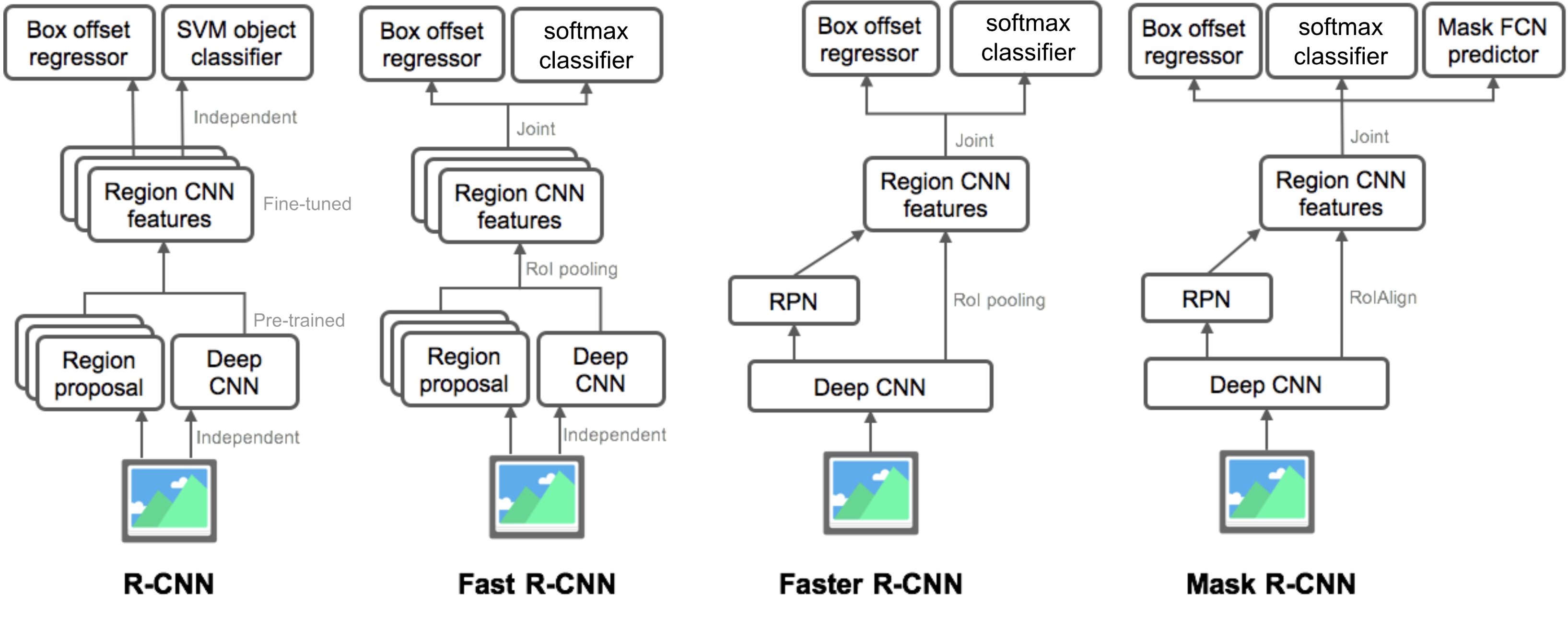
R-CNN家族。它们都是基于区域的目标检测算法。它们可以实现高精度,但对于自动驾驶等特定应用来说可能太慢。
R-CNN家族中的模型都是基于regions的。检测分为两个阶段:
(1)首先,该模型通过选择搜索或区域建议网络来提出一组感兴趣的区域。所提出的区域是稀疏的,因为潜在的边界框候选者可以是无限的。
(2) 然后分类器只处理候选区域。
这里深入细节实现R-CNN系列的检测网络.
R-CNN
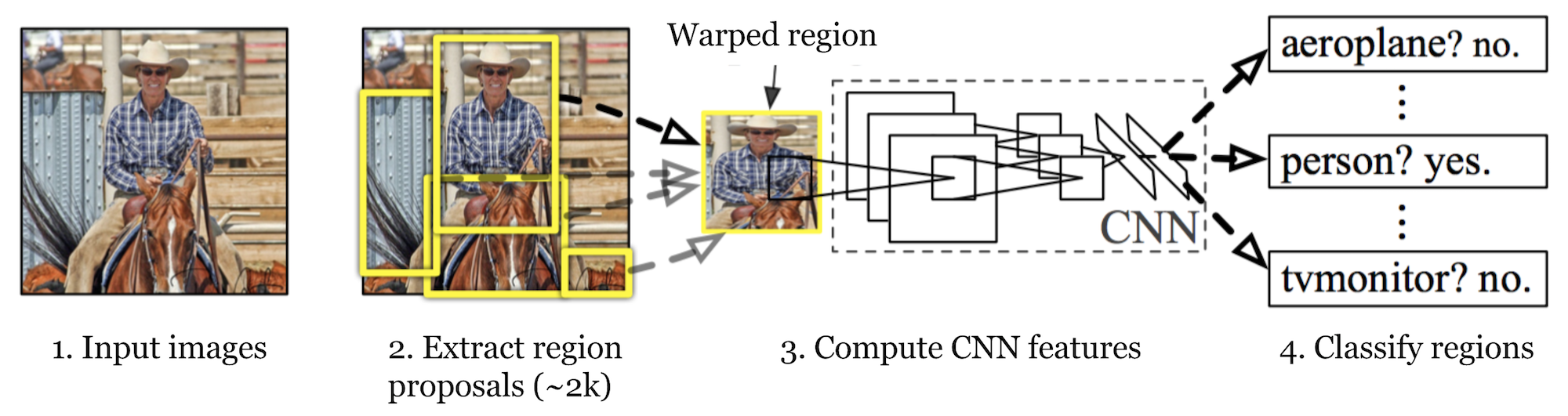
R-CNN (Girshick et al., 2014) is short for “Region-based Convolutional Neural Networks”. The main idea is composed of two steps. First, using selective search, it identifies a manageable number of bounding-box object region candidates (“region of interest” or “RoI”). And then it extracts CNN features from each region independently for classification.
选择算法(selective search)
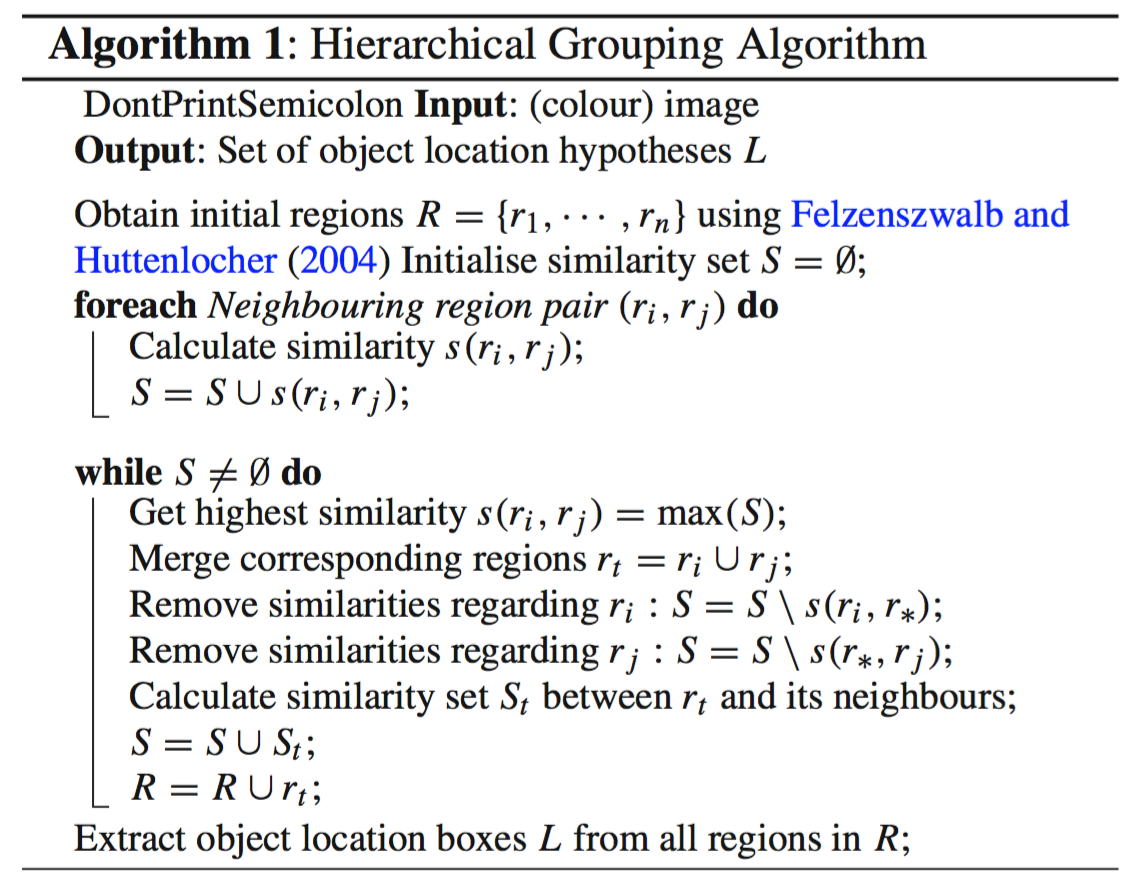
主要涉及到选择算法,用于提供可能包含对象的区域建议。它建立在图像分割输出的基础上,并使用基于区域的特征(注意:不仅仅是单个像素的属性)来进行自下而上的分层分组。
- 在初始化阶段,首先应用Felzenszwalb和Huttenlocher的基于图的图像分割算法来创建区域。
- 使用贪婪算法迭代地将区域分组在一起:
- 首先计算所有相邻区域之间的相似性。
- 将两个最相似的区域分组在一起,并计算得到的区域与其相邻区域之间的新相似性。
- 重复对最相似区域进行分组的过程(步骤2),直到整个图像变成单个区域。
可以使用颜色,材质,大小和形状作为相似度量.
流程
R-CNN流程:
使用一个预训练CNN网络,假设网络输出是K类.
通过选择性搜索提出与类别无关的感兴趣区域(每个图像约2k个候选)。这些区域可能包含目标对象,并且它们具有不同的大小。
区域被扭曲成一个固定大小.
对于第K+1类,在一个扭曲的候选区域上微调CNN(附加的一个类指的是背景(没有感兴趣的对象))。在微调阶段,我们应该使用更小的学习率,并且小批量对阳性病例进行过采样,因为大多数提出的区域只是背景。
给定每个图像区域,通过CNN的一次正向传播生成一个特征向量。然后,该特征向量输入针对每个类独立训练的二进制SVM。
正样本是IoU>=0.3的区域,而负样本是不相关的其他区域。
为了减少定位误差,训练回归模型来使用CNN特征校正边界框校正偏移上的预测检测窗口。

常用技巧
- Non-Maximum Suppression
模型可能能够为同一对象找到多个边界框。非极大值抑制有助于避免重复检测同一实例。在我们为同一对象类别获得一组匹配的边界框之后:根据置信度得分对所有边界框进行排序。丢弃置信度分数较低的方框。当存在任何剩余的边界框时,重复以下操作:贪婪地选择得分最高的边界框。然后跳过与这个边界框具有高IoU(即大于0.5)的剩余框,重复这个过程直到挑选出需要数量的bbox
非极大值抑制的方法是:先假设有6个矩形框,根据分类器的类别分类概率做排序,假设从小到大属于人脸的概率 分别为A、B、C、D、E、F。
- 从最大概率矩形框F开始,分别判断A~E与F的重叠度IOU是否大于某个设定的阈值;
- 假设B、D与F的重叠度超过阈值,那么就扔掉B、D;并标记第一个矩形框F,是我们保留下来的。
- 从剩下的矩形框A、C、E中,选择概率最大的E,然后判断E与A、C的重叠度,重叠度大于一定的阈值,那么就扔掉;并标记E是我们保留下来的第二个矩形框。
- 就这样一直重复,找到所有被保留下来的矩形框。
- Hard Negative Mining
我们将没有对象的边界框视为Negative示例。
并非所有的Negative例子都同样难以识别。例如,如果它包含纯空背景,那么它很可能是一个“容易否定的”;但是,如果盒子中包含奇怪的嘈杂纹理或部分对象,可能很难被识别为背景,这些都是“硬阴性”。严厉的反面例子很容易被错误分类。我们可以在训练循环中明确地找到那些假阳性样本,并将它们包含在训练数据中,以改进分类器。
也就说增加容易被FP的数据
通过查看R-CNN的学习步骤,您可以很容易地发现训练R-CNN模型既昂贵又缓慢,因为以下步骤需要大量工作:
- 运行选择性搜索,为每个图像提出2000个区域候选
- 为每个图像区域生成CNN特征向量(N个图像*2000)
- 整个过程分别涉及三个模型,没有太多的共享计算:用于图像分类和特征提取的卷积神经网络;用于识别目标对象的顶部SVM分类器;以及用于收紧区域边界框的回归模型。
实战
opencv实现了选择性算法.
可以参考Hulkido/RCNN: FULL Implementation of RCNN from scratch (github.com)
生成Region proposals
区域建议(Region proposals)只是图像的较小区域,可能包含我们在输入图像中搜索的对象。为了减少R-CNN中的区域建议,使用了一种称为选择性搜索的贪婪算法。
首先需要定义IoU计算1
2
3
4
5
6
7
8
9
10
11
12
13
14
15
16
17
18# calculating dimension of common area between these two boxes.
x_left = max(bb1['x1'], bb2['x1'])
y_bottom = max(bb1['y1'], bb2['y1'])
x_right = min(bb1['x2'], bb2['x2'])
y_top = min(bb1['y2'], bb2['y2'])
# if there is no overlap output 0 as intersection area is zero.
if x_right < x_left or y_bottom < y_top:
return 0.0
# calculating intersection area.
# 计算交集
intersection_area = (x_right - x_left) * (y_top - y_bottom)
# individual areas of both these bounding boxes.
# 计算各自区域面积
bb1_area = (bb1['x2'] - bb1['x1']) * (bb1['y2'] - bb1['y1'])
bb2_area = (bb2['x2'] - bb2['x1']) * (bb2['y2'] - bb2['y1'])
# union area = area of bb1_+ area of bb2 - intersection of bb1 and bb2.
# 并集就是各自之和减去交集
iou = intersection_area / float(bb1_area + bb2_area - intersection_area)
遍历选择性搜索得到的区域,计算每个区域与对应bbox(bounding box)的IoU.
然后将iou大于阈值(这里设置为0.7)的定为region proposal,同时resize这个区域建议.
本身应该是warp,但我觉得差别不大.另外region proposal和ROI差别其实也不大,有说法是region proposal是对图像而言的,roi是针对feature map上的.

1
2
3
4
5
6
7
8
9
10
11
12
13
14
15
16
17
18
19
20
21
22
23
24
25
26
27
28
29
30
31
32
33
34
35
36
37
38import cv2
cv2.setUseOptimized(True);
ss = cv2.ximgproc.segmentation.createSelectiveSearchSegmentation()
ss.setBaseImage(image) # setting given image as base image
ss.switchToSelectiveSearchFast() # running selective search on bae image
ssresults = ss.process() # processing to get the outputs
imout = image.copy()
counter = 0
falsecounter = 0
flag = 0
fflag = 0
bflag = 0
for e,result in enumerate(ssresults):
if e < 2000 and flag == 0: # till 2000 to get top 2000 regions only
for gtval in gtvalues:
x,y,w,h = result
iou = get_iou(gtval,{"x1":x,"x2":x+w,"y1":y,"y2":y+h}) # calculating IoU for each of the proposed regions
if counter < 30: # getting only 30 psoitive examples
if iou > 0.70: # IoU or being positive is 0.7
timage = imout[x:x+w,y:y+h]
resized = cv2.resize(timage, (224,224), interpolation = cv2.INTER_AREA)
train_images.append(resized)
train_labels.append(1)
counter += 1
else :
fflag =1 # to insure we have collected all psotive examples
if falsecounter <30: # 30 negatve examples are allowed only
if iou < 0.3: # IoU or being negative is 0.3
timage = imout[x:x+w,y:y+h]
resized = cv2.resize(timage, (224,224), interpolation = cv2.INTER_AREA)
train_images.append(resized)
train_labels.append(0)
falsecounter += 1
else :
bflag = 1 #to ensure we have collected all negative examples
if fflag == 1 and bflag == 1:
print("inside")
flag = 1 # to signal the complition of data extaction from a particular image
上面一共最多遍历生成的2000个ROI,选取其中的正例(超过阈值)的30,负例30.
下面是一张图像与其得到的正例和负例


使用CNN模型二分类
一般直接使用预训练模型,这里使用keras,加载VGG16模型.这里只做目标是否在而不做具体分类,所以输出单个值作为二分类.1
2
3
4
5
6
7
8
9
10
11
12
13vgg = tf.keras.applications.vgg16.VGG16(include_top=True, weights='imagenet', input_tensor=None, input_shape=None, pooling=None, classes=1000)
for layer in vgg.layers[:-2]:
layer.trainable = False
x = vgg.get_layer('fc2')
last_output = x.output
x = tf.keras.layers.Dense(1,activation = 'sigmoid')(last_output)
model = tf.keras.Model(vgg.input,x)
model.compile(optimizer = "adam",
loss = 'binary_crossentropy',
metrics = ['acc'])
model.summary()
model.fit(X_new,Y_new,batch_size = 64,epochs = 3, verbose = 1,validation_split=.05,shuffle = True)
预训练模型提取特征再使用SVM二分类
原文中为每一类使用了一个二分类的SVM(毕竟一般的一个SVM只能二分类)
可以再上面的预训练模型只使用特征提取层,然后加个SVM
bbox regression
最后需要求的bbox的回归用于修正误差.
回归后得到四个参数,即x,y中心点偏移量和高、宽缩放因子,利用这四个参数对剩余的高质量目标建议框进行调整,取得分最高的称为Bounding Box,完成定位任务。

如图,x,y坐标的修正由p~w~d~x~(p)+p~x~,而w,h由p~w~exp(d~w~(p))修正,已知t~i~函数,需要求d~i~(p)的回归值.1
2
3
4
5
6
7
8
9
10
11
12
13
14
15
16
17
18
19
20curr_iou = iou([gta[bbox_num, 0], gta[bbox_num, 2], gta[bbox_num, 1], gta[bbox_num, 3]], [x1_anc, y1_anc, x2_anc, y2_anc])
# calculate the regression targets if they will be needed
if curr_iou > best_iou_for_bbox[bbox_num] or curr_iou > C.rpn_max_overlap:
cx = (gta[bbox_num, 0] + gta[bbox_num, 1]) / 2.0 # center point of bbox
cy = (gta[bbox_num, 2] + gta[bbox_num, 3]) / 2.0
cxa = (x1_anc + x2_anc)/2.0 # center point of anchor box which scales to resized image
cya = (y1_anc + y2_anc)/2.0
tx = (cx - cxa) / (x2_anc - x1_anc) # regression targets
ty = (cy - cya) / (y2_anc - y1_anc)
tw = np.log((gta[bbox_num, 1] - gta[bbox_num, 0]) / (x2_anc - x1_anc))
th = np.log((gta[bbox_num, 3] - gta[bbox_num, 2]) / (y2_anc - y1_anc))
if img_data['bboxes'][bbox_num]['class'] != 'bg':
# all GT boxes should be mapped to an anchor box, so we keep track of which anchor box was best
if curr_iou > best_iou_for_bbox[bbox_num]:
best_anchor_for_bbox[bbox_num] = [jy, ix, anchor_ratio_idx, anchor_size_idx]
best_iou_for_bbox[bbox_num] = curr_iou
best_x_for_bbox[bbox_num,:] = [x1_anc, x2_anc, y1_anc, y2_anc]
best_dx_for_bbox[bbox_num,:] = [tx, ty, tw, th]
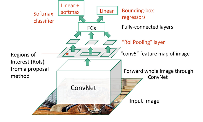
Fast R-CNN
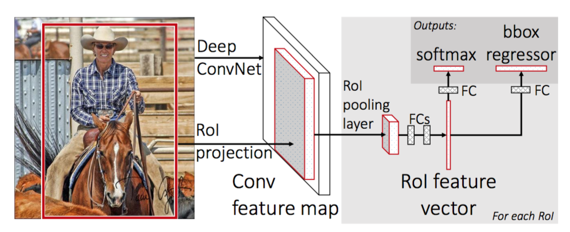
为了使R-CNN更快,Girshick(2015)通过将三个独立的模型统一到一个联合训练的框架中并增加共享计算结果(称为Fast R-CNN)来改进训练过程。
不同于R-CNN对于每个region proposals提取特征,,而是将它们聚合到整个图像上的一个 CNN 前向传递中,并且region proposals共享此特征矩阵。然后,将相同的特征矩阵分支出来,用于学习对象分类器和边界框回归器。总之,计算共享加速了R-CNN。
ROI Pooling
1 | x = torch.arange(16).reshape(1,1,4,4) |
1
2
3
4
5
6
7
8
9
10
11
12
13
14
15
16def roi_pooling(features, rois, output_size):
# features: 输入特征图 (N, C, H, W)
# rois: 区域候选框 (N, 4) 其中每行表示一个候选框的坐标 (x1, y1, x2, y2)
# output_size: ROI Pooling的输出尺寸 (H', W')
num_rois = rois.size(0)
output = torch.zeros(num_rois, features.size(1), output_size, output_size)
for i in range(num_rois):
roi = rois[i]
x1, y1, x2, y2 = roi
roi_features = features[:, :, y1:y2 + 1, x1:x2 + 1]
roi_features = F.adaptive_max_pool2d(roi_features, output_size)
output[i] = roi_features
return output
上面的算法其实使用的是pytorch的adaptive_max_pool2d,这两个东西并不一样,但很多简易实现就是利用了这个函数
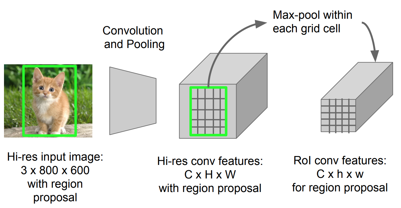
由于要进行分类和回归(都使用一个FC),需要一个固定大小的输入.由于此时输入已经成了可训练的feature map而不是直接的图像,需要一个可微分的操作.
RoI 池化类似于 max-pooling。说白了就是将原本的region proposals分成hxw的grid,这里的h,w就是后面fc需要的输入,在每个grid中做max pooling1
2
3
4
5
6
7
8
9
10
11
12
13
14
15
16
17
18
19
20
21
22
23
24
25
26
27
28
29
30
31class FastRCNN(nn.Module):
def __init__(self, num_classes):
super().__init__()
self.num_classes = num_classes
vgg = torchvision.models.vgg19_bn(pretrained=True)
self.features = nn.Sequential(*list(vgg.features.children())[:-1])
self.roipool = ROIPooling(output_size=(7, 7))
#roipooling之后得到B,C,7,7直接
self.output = nn.Sequential(*list(vgg.classifier.children())[:-1])
self.prob = nn.Linear(4096, num_classes+1)
self.loc = nn.Linear(4096, 4 * (num_classes + 1))
self.cat_loss = nn.CrossEntropyLoss()
self.loc_loss = nn.SmoothL1Loss()
def forward(self, img, rois, roi_idx):
res = self.features(img)
res = self.roipool(res, rois, roi_idx)
res = res.view(res.shape[0], -1)
features = self.output(res)
prob = self.prob(features)
loc = self.loc(features).view(-1, self.num_classes+1, 4)
return prob, loc
def loss(self, prob, bbox, label, gt_bbox, lmb=1.0):
loss_cat = self.cat_loss(prob, label)
lbl = label.view(-1, 1, 1).expand(label.size(0), 1, 4)
mask = (label != 0).float().view(-1, 1, 1).expand(label.shape[0], 1, 4)
loss_loc = self.loc_loss(gt_bbox * mask, bbox.gather(1, lbl).squeeze(1) * mask)
loss = loss_cat + lmb * loss_loc
return loss, loss_cat, loss_loc
- 首先,在图像分类任务上预训练卷积神经网络。
- 通过选择性搜索提出区域建议(每张图像~2k个候选者)。
- 更改预训练的 CNN:
- 将预训练 CNN 的最后一个最大池化层替换为 RoI 池化层。RoI 池化层输出区域建议的固定长度特征向量。共享 CNN 计算很有意义,因为相同图像的许多区域建议是高度重叠的。
- 将最后一个全连接层和最后一个 softmax 层(K 类)替换为全连接层和 K + 1 类上的 softmax。
- 最后,模型分为两个输出:K + 1 类的 softmax 估计器(与 R-CNN 相同,+1 是“背景”类),输出每个 RoI 的离散概率分布。一个边界框回归模型,用于预测每个 K 类相对于原始 RoI 的偏移量。
损失函数有分类损失和回归损失,回归损失用于计算bouding box的回归损失,可使用L1损失。
在Fast RCNN中,改进并不显著,因为区域提案是由另一个模型单独生成的,而且非常耗时。
流程
首先,在图像分类任务上预训练卷积神经网络。
通过选择性搜索提出区域建议(每张图像~2k个候选者)。
更改预训练的 CNN:将预训练 CNN 的最后一个最大池化层替换为 RoI 池化层。
RoI 池化层输出区域建议的固定长度特征向量。共享 CNN 计算很有意义,因为相同图像的许多区域建议是高度重叠的。
将最后一个全连接层和最后一个 softmax 层(K 类)替换为全连接层和 K + 1 类上的 softmax。最后,模型分支为两个输出层:K + 1 类的 softmax 估计器(与 R-CNN 相同,+1 是“背景”类),输出每个 RoI 的离散概率分布。一个边界框回归模型,用于预测每个 K 类相对于原始 RoI 的偏移量。
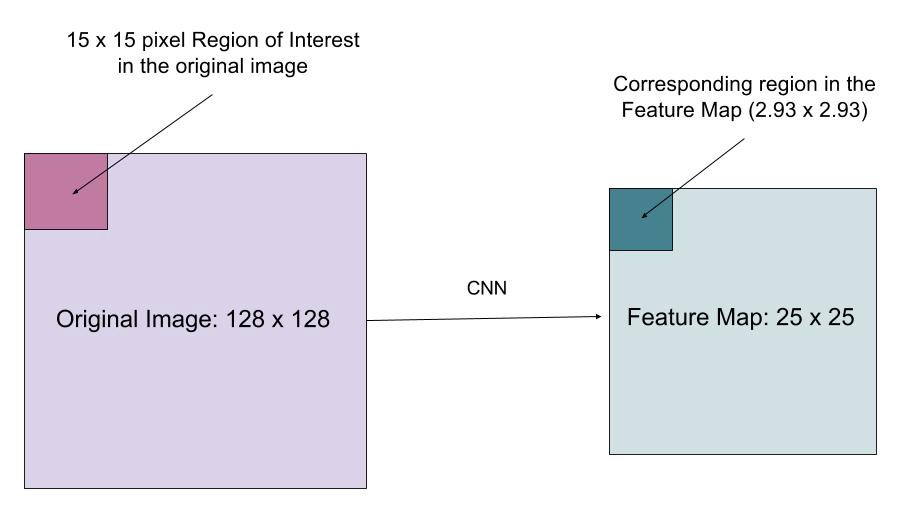
其中关键是如何利用选择搜索得到的region proposals映射到通过CNN得到的feature map上,这样就只用在整个图像上进行一次CNN而不是单独在每个region proposal上滤波.如果只进行一次滤波,如何准确地将输入图像的一个区域投影到卷积特征图的一个区域上,此外还有ROI Pooling得到固定的ROI区域也是关键.
SPPNet介绍了 ROI Projection,看起来貌似就是算回去,不过在设计CNN时,padding = kernel_size/2这样避免计算复杂

Loss包括分类损失和bouding box回归损失

Faster RNN
重点说一下faster rcnn
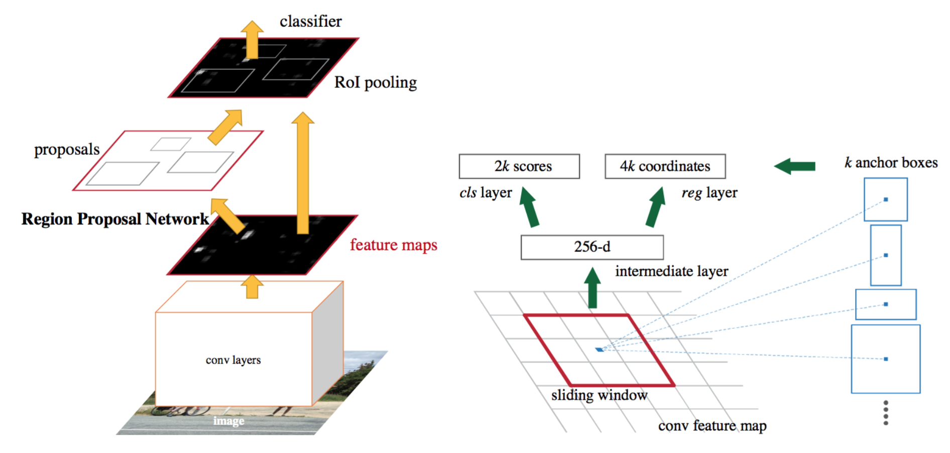
将选择性搜索算法(也就是用于生成region proposals的算法)融合到深度学习模型中

比如下面将一张图像通过一个模型1
2
3
4
5
6
7
8
9
10
11
12
13
14
15
16
17
18
19
20
21
22
23
24
25
26
27
28
29
30
31
32
33
34
35
36
37
38
39
40
41
42
43
44
45ef nn_base(input_tensor=None, trainable=False):
# Determine proper input shape
if K.image_data_format() == 'channels_first':
input_shape = (3, None, None)
else:
input_shape = (None, None, 3)
if input_tensor is None:
img_input = Input(shape=input_shape)
else:
if not K.is_keras_tensor(input_tensor):
img_input = Input(tensor=input_tensor, shape=input_shape)
else:
img_input = input_tensor
if K.image_data_format() == 'channels_last':
bn_axis = 3
else:
bn_axis = 1
x = ZeroPadding2D((3, 3))(img_input)
x = Convolution2D(64, (7, 7), strides=(2, 2), name='conv1', trainable = trainable)(x)
x = FixedBatchNormalization(axis=bn_axis, name='bn_conv1')(x)
x = Activation('relu')(x)
x = MaxPooling2D((3, 3), strides=(2, 2))(x)
x = conv_block(x, 3, [64, 64, 256], stage=2, block='a', strides=(1, 1), trainable = trainable)
x = identity_block(x, 3, [64, 64, 256], stage=2, block='b', trainable = trainable)
x = identity_block(x, 3, [64, 64, 256], stage=2, block='c', trainable = trainable)
x = conv_block(x, 3, [128, 128, 512], stage=3, block='a', trainable = trainable)
x = identity_block(x, 3, [128, 128, 512], stage=3, block='b', trainable = trainable)
x = identity_block(x, 3, [128, 128, 512], stage=3, block='c', trainable = trainable)
x = identity_block(x, 3, [128, 128, 512], stage=3, block='d', trainable = trainable)
x = conv_block(x, 3, [256, 256, 1024], stage=4, block='a', trainable = trainable)
x = identity_block(x, 3, [256, 256, 1024], stage=4, block='b', trainable = trainable)
x = identity_block(x, 3, [256, 256, 1024], stage=4, block='c', trainable = trainable)
x = identity_block(x, 3, [256, 256, 1024], stage=4, block='d', trainable = trainable)
x = identity_block(x, 3, [256, 256, 1024], stage=4, block='e', trainable = trainable)
x = identity_block(x, 3, [256, 256, 1024], stage=4, block='f', trainable = trainable)
return x
提出了Region Proposal Networks
Region Proposal Networks
主要更改就是对于roi projection,之前还是在原图上使用ss得到region proposals然后映射到feature map上,现在用区域提案网络 (RPN)替代,其他部分不变.
RPN,简单地说,它是一个小型的全卷积网络,它接受feature map,并输出一组区域和每个区域的“objectiveness”分数(该区域包含对象的可能性)。

首先使用一个cnn模型提取特征得到feature map,而RPN就会利用这个feature map,并且提出了anchor boxes概念,在feature map上使用一个大小为3x3的sliding window,在sliding window移动到一个位置的时候生成多个不同大小的anchor boxes.
在生成相关数据的时候,对于一个feature map,由于它已经经过多次卷积包含许多信息,在这个feature map上生成anchor box.1
2
3
4# initialise empty output objectives
y_rpn_overlap = np.zeros((output_height, output_width, num_anchors))
y_is_box_valid = np.zeros((output_height, output_width, num_anchors))
y_rpn_regr = np.zeros((output_height, output_width, num_anchors * 4))
其中num_anchors设定为9,包含三种不同大小以及比例的的anchor box.
y_rpn_overlap表示这个anchor box是否包含物体,在生成数据时会将与bbox的iou大于一个阈值(比如0.7)的作为pos,小于一个阈值(0.3)作为neg表示不包含物体,也就是背景.在代码中,如果一个大于0.7的anchor box都没有那就直接取与bounding box的iou最大的作为包含物体的anchor box正例.
y_is_box_valid表示所有正负例anchor box,去掉iou在0.3~0.7的,认为这些anchor box不明显.一般这个值会设置一个固定值,注意,生成的anchor box如果是pos,只表示其与其中一个或多个bbox的iou大于阈值,并不能知道其与哪个物体位置更相近.
y_rpn_regr表示anchor box的具体位置1
y_rpn_cls, y_rpn_regr = calc_rpn(C, img_data_aug, width, height, resized_width, resized_height, img_length_calc_function)
1
2
y_rpn_cls = np.concatenate([y_is_box_valid, y_rpn_overlap], axis=1)
y_rpn_regr = np.concatenate([np.repeat(y_rpn_overlap, 4, axis=1), y_rpn_regr], axis=1)
计算rpn输出时为什么要concat这些数据?这是在代码实现层面的事,calc_rpn计算得到固定个数的正负例作为训练数据1
2
3
4
5
6
7
8
9
10
11
12
13
14
15
16
17
18
19# one issue is that the RPN has many more negative than positive regions, so we turn off some of the negative
# regions. We also limit it to 256 regions.
num_regions = 256
# 对于一张图 只选取256个anchor box
# change from len(pos_locs[0]) to len(pos_locs)
if len(pos_locs) > num_regions/2:
val_locs = random.sample(range(len(pos_locs[0])), len(pos_locs[0]) - num_regions/2)
y_is_box_valid[0, pos_locs[0][val_locs], pos_locs[1][val_locs], pos_locs[2][val_locs]] = 0
num_pos = num_regions/2
if len(neg_locs) + num_pos > num_regions:
val_locs = random.sample(range(len(neg_locs[0])), len(neg_locs[0]) - num_pos)
y_is_box_valid[0, neg_locs[0][val_locs], neg_locs[1][val_locs], neg_locs[2][val_locs]] = 0
# 这里 y_rpn_regr 为什么要concatenate四个正例?
y_rpn_cls = np.concatenate([y_is_box_valid, y_rpn_overlap], axis=1)
y_rpn_regr = np.concatenate([np.repeat(y_rpn_overlap, 4, axis=1), y_rpn_regr], axis=1)
# y_rpn_cls (1, 18, 26, 35)
# y_rpn_regr (1, 72, 26, 35)1
2rpn_accuracy_rpn_monitor = []
rpn_accuracy_for_epoch = []
训练代码中设计了rpn_accuracy_rpn_monitor和rpn_accuracy_rpn_monitor,前者会在处理过的图像达到一定数量后计算rpn的准确率,也就是生成的roi是否总是正例.
后者会在每次epoch完后计算mean loss和acc,因为在这个目标检测任务中,每次epoch的batch_size并不是像其他任务取多张图像,而是每次epoch中又取epoch_length,每次取一张图片.
问题1
RPN如何设计的,3x3的sliding window有什么用,如果是为了生成anchor box,有必要设计一个sliding window吗?
在通过一个预训练模型的feature层后(比如vgg,resnet,inception等等),再使用一个3x3的sliding window,通道数256(可以理解为再聚合一下信息),然后在原本的feature map上针对每个pixel生成多个anchor box.
遍历一个图像上的所有bbox,看它与生成的anchor box的iou,取一个大于0.7的最大的anchor box的pos,其余的小于0.3的是neg.
首先将feature map做一次3x3卷积,在进行全卷积的输出分别得到针对一个anchor box的二分类以及修正坐标(坐标回归)1
2
3
4
5
6
7
8
9
10
11def rpn(base_layers,num_anchors):
# important! same width,hight
x = Convolution2D(512, (3, 3), padding='same', activation='relu', kernel_initializer='normal', name='rpn_conv1')(base_layers)
# get class and regr output
# fully convolution
x_class = Convolution2D(num_anchors, (1, 1), activation='sigmoid', kernel_initializer='uniform', name='rpn_out_class')(x)
x_regr = Convolution2D(num_anchors * 4, (1, 1), activation='linear', kernel_initializer='zero', name='rpn_out_regress')(x)
return [x_class, x_regr, base_layers]
然后利用roi pooling以及classifier输出针对于21类的概率和20类回归坐标1
2
3
4
5
6
7
8
9
10
11
12
13
14
15
16
17
18
19
20def classifier(base_layers, input_rois, num_rois, nb_classes = 21, trainable=False):
# compile times on theano tend to be very high, so we use smaller ROI pooling regions to workaround
if K.backend() == 'tensorflow':
pooling_regions = 14
input_shape = (num_rois,14,14,1024)
elif K.backend() == 'theano':
pooling_regions = 7
input_shape = (num_rois,1024,7,7)
out_roi_pool = RoiPoolingConv(pooling_regions, num_rois)([base_layers, input_rois])
out = classifier_layers(out_roi_pool, input_shape=input_shape, trainable=True)
out = TimeDistributed(Flatten())(out)
out_class = TimeDistributed(Dense(nb_classes, activation='softmax', kernel_initializer='zero'), name='dense_class_{}'.format(nb_classes))(out)
# note: no regression target for bg class
out_regr = TimeDistributed(Dense(4 * (nb_classes-1), activation='linear', kernel_initializer='zero'), name='dense_regress_{}'.format(nb_classes))(out)
return [out_class, out_regr]
这样就训练三个模型1
2
3
4
5model_rpn = Model(img_input, rpn[:2])
model_classifier = Model([img_input, roi_input], classifier)
# this is a model that holds both the RPN and the classifier, used to load/save weights for the models
model_all = Model([img_input, roi_input], rpn[:2] + classifier)
rpn损失计算,1
2
3
4
5
6
7
8
9
10
11
12
13
14
15
16
17
18
19
20
21
22
23
24
25
26
27def rpn_loss_regr(num_anchors):
def rpn_loss_regr_fixed_num(y_true, y_pred):
if K.image_data_format() == 'channels_first':
x = y_true[:, 4 * num_anchors:, :, :] - y_pred
x_abs = K.abs(x)
x_bool = K.less_equal(x_abs, 1.0)
return lambda_rpn_regr * K.sum(
y_true[:, :4 * num_anchors, :, :] * (x_bool * (0.5 * x * x) + (1 - x_bool) * (x_abs - 0.5))) / K.sum(epsilon + y_true[:, :4 * num_anchors, :, :])
else:
x = y_true[:, :, :, 4 * num_anchors:] - y_pred
x_abs = K.abs(x)
x_bool = K.cast(K.less_equal(x_abs, 1.0), tf.float32)
return lambda_rpn_regr * K.sum(
y_true[:, :, :, :4 * num_anchors] * (x_bool * (0.5 * x * x) + (1 - x_bool) * (x_abs - 0.5))) / K.sum(epsilon + y_true[:, :, :, :4 * num_anchors])
return rpn_loss_regr_fixed_num
def rpn_loss_cls(num_anchors):
def rpn_loss_cls_fixed_num(y_true, y_pred):
if K.image_data_format() == 'channels_last':
return lambda_rpn_class * K.sum(y_true[:, :, :, :num_anchors] * K.binary_crossentropy(y_pred[:, :, :, :], y_true[:, :, :, num_anchors:])) / K.sum(epsilon + y_true[:, :, :, :num_anchors])
else:
return lambda_rpn_class * K.sum(y_true[:, :num_anchors, :, :] * K.binary_crossentropy(y_pred[:, :, :, :], y_true[:, num_anchors:, :, :])) / K.sum(epsilon + y_true[:, :num_anchors, :, :])
return rpn_loss_cls_fixed_num
计算得到P_rpn也就是在feature maps上通过RPN网络得到的300个anchor boxes坐标以及sigmoid分数(表示是否包含物体)
然后调整anchor box使其区域在feature map内,1
2
3
4
5
6
7
8
9
10
11
12
13
14
15
16
17
18
19anchor_x = (anchor_size * anchor_ratio[0])/C.rpn_stride
anchor_y = (anchor_size * anchor_ratio[1])/C.rpn_stride
X, Y = np.meshgrid(np.arange(cols),np. arange(rows))
A[0, :, :, curr_layer] = X - anchor_x/2
A[1, :, :, curr_layer] = Y - anchor_y/2
A[2, :, :, curr_layer] = anchor_x
A[3, :, :, curr_layer] = anchor_y
A[2, :, :, curr_layer] = np.maximum(1, A[2, :, :, curr_layer])
A[3, :, :, curr_layer] = np.maximum(1, A[3, :, :, curr_layer])
A[2, :, :, curr_layer] += A[0, :, :, curr_layer]
A[3, :, :, curr_layer] += A[1, :, :, curr_layer]
A[0, :, :, curr_layer] = np.maximum(0, A[0, :, :, curr_layer])
A[1, :, :, curr_layer] = np.maximum(0, A[1, :, :, curr_layer])
A[2, :, :, curr_layer] = np.minimum(cols-1, A[2, :, :, curr_layer])
A[3, :, :, curr_layer] = np.minimum(rows-1, A[3, :, :, curr_layer])
此外就是NMS了,输入是anchor box shape是(h*w*9,4)以及对应的一个概率对应着(h*w*9)值在0-1之间表示对应anchor box包含物体的概率.将从一个图像中得到的所有anchor box经过NMS,这样一张图像中的anchor box最多也就一定数量(比如300)了.
然后对于这些anchor box,计算与其iou最大的bbox,要求最大的iou大于一定值(比如0.7),那么这个就是roi,其类别就是对应bbox类别,并且设置其位置(修正位置).
然后设置一定数量需要的rois,尽量均匀分正负例1
2
3
4
5
6
7
8
9
10
11
12
13
14
15
16
17
18
19
20
21
22
23
24
25
26
27
28
29
30
31
32
33
34
35
36
37
38
39
40
41
42
43
44
45
46
47
48
49
50
51
52
53
54
55
56
57
58
59
60
61
62
63
64
65
66
67
68def non_max_suppression_fast(boxes, probs, overlap_thresh=0.9, max_boxes=300):
# code used from here: http://www.pyimagesearch.com/2015/02/16/faster-non-maximum-suppression-python/
# if there are no boxes, return an empty list
if len(boxes) == 0:
return []
# grab the coordinates of the bounding boxes
x1 = boxes[:, 0]
y1 = boxes[:, 1]
x2 = boxes[:, 2]
y2 = boxes[:, 3]
np.testing.assert_array_less(x1, x2)
np.testing.assert_array_less(y1, y2)
# if the bounding boxes integers, convert them to floats --
# this is important since we'll be doing a bunch of divisions
if boxes.dtype.kind == "i":
boxes = boxes.astype("float")
# initialize the list of picked indexes
pick = []
# calculate the areas
area = (x2 - x1) * (y2 - y1)
# sort the bounding boxes
idxs = np.argsort(probs)
# keep looping while some indexes still remain in the indexes
# list
while len(idxs) > 0:
# grab the last index in the indexes list and add the
# index value to the list of picked indexes
last = len(idxs) - 1
i = idxs[last]
pick.append(i)
# find the intersection
xx1_int = np.maximum(x1[i], x1[idxs[:last]])
yy1_int = np.maximum(y1[i], y1[idxs[:last]])
xx2_int = np.minimum(x2[i], x2[idxs[:last]])
yy2_int = np.minimum(y2[i], y2[idxs[:last]])
ww_int = np.maximum(0, xx2_int - xx1_int)
hh_int = np.maximum(0, yy2_int - yy1_int)
area_int = ww_int * hh_int
# find the union
area_union = area[i] + area[idxs[:last]] - area_int
# compute the ratio of overlap
overlap = area_int / (area_union + 1e-6)
# delete all indexes from the index list that have
idxs = np.delete(idxs, np.concatenate(([last],
np.where(overlap > overlap_thresh)[0])))
if len(pick) >= max_boxes:
break
# return only the bounding boxes that were picked using the integer data type
boxes = boxes[pick].astype("int")
probs = probs[pick]
return boxes, probs
大致逻辑是选取probs最大的(也就是通过RPN算出来包含物体概率最大的anchor box),计算其与剩余的anchor box的iou,去掉大于某个阈值(比如0.9)的,然后再重复,选择剩下来的probs最大的anchor box.一共选择固定数量的anchor box.返回相应的boxes以及probs.
可以看看这个Faster R-CNN 论文阅读记录(一):概览 - 知乎 (zhihu.com)
一文读懂Faster RCNN - 知乎 (zhihu.com)
Mask R-CNN
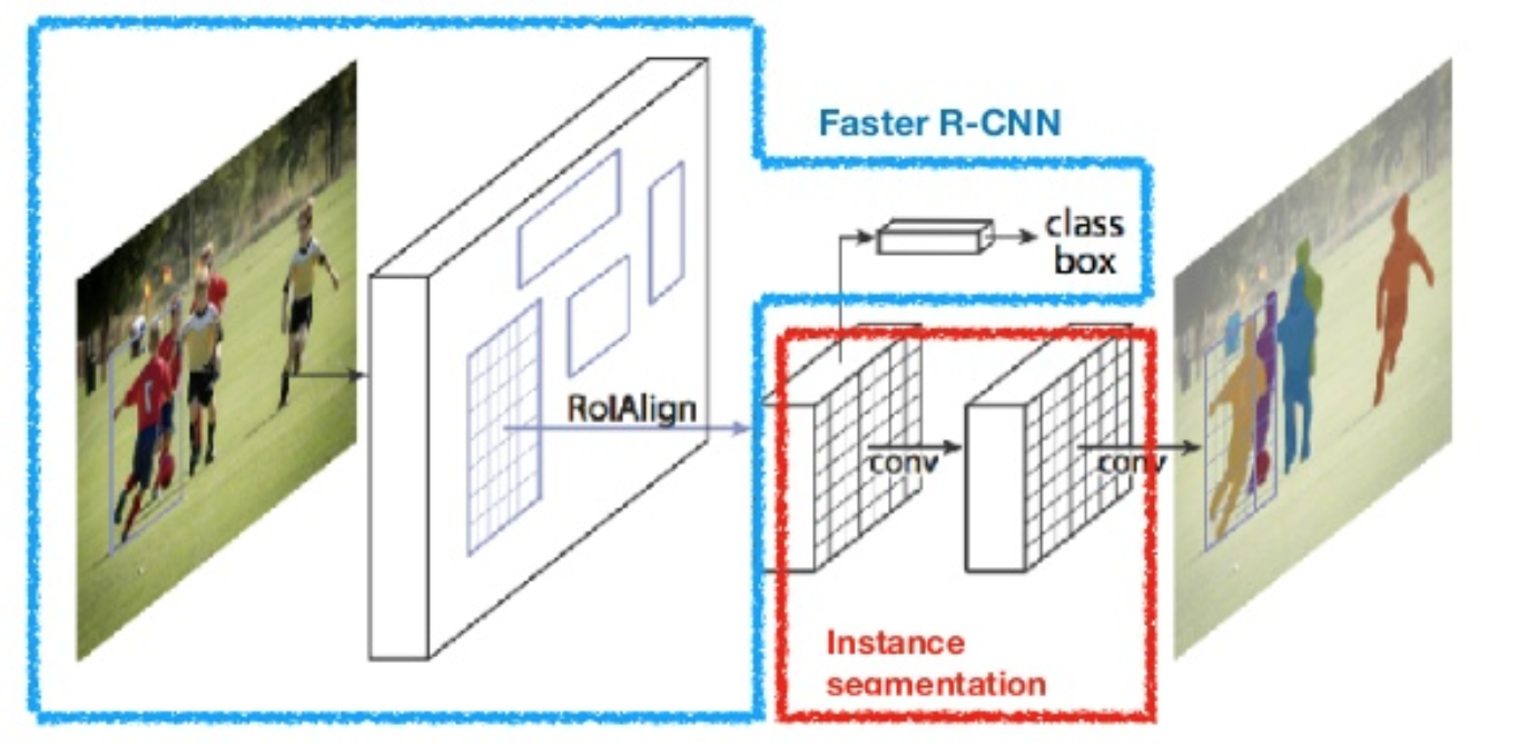
主要是提出了ROIAlign将模型用于实例分割中,可以与原先的任务并行,
RoIAlign 层旨在修复 RoI 池化中由量化(quantization)引起的位置错位。RoIAlign 删除哈希量化,例如,使用 x/16 而不是 [x/16],以便提取的特征可以与输入像素正确对齐。双线性插值用于计算输入中的浮点位置值。
作者认为Faster RCNN中ROI pooling的取整(quantization )操作会使得定位不准确
这种quantization还体现在proposals(在原图上)映射到特征层上的操作,因为这会导致不对准,对于detection任务有较大影响,

上图蓝框就是proposals到feature map上的框,没有取整.然后在每个roi中选择采样点计算这些采样的均值即为每个roi的值
可以看看这篇文章【精选】Mask R-CNN网络详解_mask rcnn详解-CSDN博客
Region-based Fully Convolutional Network (R-FCN)

可以了解一下全卷积网络(13.11. 全卷积网络 — 动手学深度学习 2.0.0 documentation (d2l.ai)).1×1卷积层通常用于调整网络层的通道数量和控制模型复杂性
全卷积网络先使用卷积神经网络抽取图像特征,然后通过1×1卷积层将通道数变换为类别个数,最后通过转置卷积层将特征图的高和宽变换为输入图像的尺寸。输出的类别预测与输入图像在像素级别上具有一一对应关系:通道维的输出即该位置对应像素的类别预测
R-FCN核心操作是将ROI pooling改为了position-sensitive score maps.而且原本在ROI pooling之后的卷积层和全连接层(被认为是位置不敏感的操作,这种操作会影响目标检测的精度而且浪费神经网络的分类能力),所以文章将全部操作改为卷积

大致流程如下:
- 首先选择一张需要处理的图片,并对这张图片进行相应的预处理操作;
- 接着,我们将预处理后的图片送入一个预训练好的分类网络中(这里使用了ResNet-101网络的Conv4之前的网络),固定其对应的网络参数;
- 接着,在预训练网络的最后一个卷积层获得的feature map上存在3个分支,第1个分支就是在该feature map上面进行RPN操作,获得相应的ROI;第2个分支就是在该feature map上获得一个K*K*(C+1)维的位置敏感得分映射(position-sensitive score map),用来进行分类;第3个分支就是在该feature map上获得一个4*K*K维的位置敏感得分映射,用来进行回归;
- 最后,在K*K*(C+1)维的位置敏感得分映射和4KK维的位置敏感得分映射上面分别执行位置敏感的ROI池化操作(Position-Sensitive Rol Pooling,这里使用的是平均池化操作),获得对应的类别和位置信息。
具体来说,通过一个CNN网络后得到feature map,一方面使用全卷积网络将通道数调整为k*k*(C+1)(对于分类任务),此外也需要一个RPN网络,用于提取roi区域,得到roi之后,将每个roi分为k*k个bins,这个时候每个bin就对应一个类别中k*k个通道之一,池化操作也就在这个通道上进行操作.i,j表示每个roi中的某个bin,c表示通道数,其中n表示bin中的像素数,相当于对于某个类别c中的某个bin,计算得到的scores(其实就是一个通道的和)除以bin中的像素数量.论文中的所谓vote就是简单地使用均值得到k*k个position-sensitive scores.
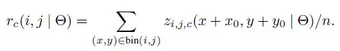
然后按此计算某个类别的池化值,也就是k*k个bin的值的和,每个bin是映射在某个score map上的avg pooling.

得到C+1个值然后做softmax作为评价交叉熵巡视以及对roi的排名.

Summary of R-CNN family
以上都是two-stage detector,另一种不同的方法跳过区域建议阶段,直接在可能位置的密集采样上运行检测。这就是单阶段目标检测算法的工作原理。这更快、更简单,但可能会降低performance。
在One-stage中对象检测是一个简单的回归问题,需要输入并学习概率类和边界框坐标。YOLO、YOLO v2、SSD、RetinaNet等属于一个相位检测器。对象检测是图像分类的一种高级形式,其中神经网络预测图像中的对象,并以边界框的形式引起人们的注意。
论文相关
Rich feature hierarchies for accurate object detection and semantic segmentation
2014年的论文,为后面RCNN系列目标检测方法奠定基础
abs
Object detection performance, as measured on the canonical PASCAL VOC dataset, has plateaued in the last few years.The best-performing methods are complex ensemble systems that typically combine multiple low-level image features with high-level context.In this paper, we propose a simple and scalable detection algorithm that improves mean average precision (mAP) by more than 30% relative to the previous best result on VOC 2012—achieving a mAP of 53.3%.Our approach combines two key insights: (1) one can apply high-capacity convolutional neural networks (CNNs) to bottom-up region proposals in order to localize and segment objects and (2) when labeled training data is scarce, supervised pre-training for an auxiliary task, followed by domain-specific fine-tuning, yields a significant performance boost.
Mask-RCNN
abs
We present a conceptually simple, flexible, and general framework for object instance segmentation. Our approach efficiently detects objects in an image while simultaneously generating a high-quality segmentation mask for each instance.
The method, called Mask R-CNN, extends Faster R-CNN by adding a branch for predicting an object mask in parallel with the existing branch for bounding box recognition. Mask R-CNN is simple to train and adds only a small overhead to Faster R-CNN, running at 5 fps.
Moreover, Mask R-CNN is easy to generalize to other tasks, e.g., allowing us to estimate human poses in the same framework. We show top results in all three tracks of the COCO suite of challenges, including instance segmentation, boundingbox object detection, and person keypoint detection.
R-FCN
abs
We present region-based, fully convolutional networks for accurate and efficient object detection. In contrast to previous region-based detectors such as Fast/Faster R-CNN [6, 18] that apply a costly per-region subnetwork hundreds of times, our region-based detector is fully convolutional with almost all computation shared on the entire image.
To achieve this goal, we propose position-sensitive score maps to address a dilemma between translation-invariance in image classification and translation-variance in object detection.
Our method can thus naturally adopt fully convolutional image classifier backbones, such as the latest Residual Networks (ResNets) [9], for object detection. We show competitive results on the PASCAL VOC datasets (e.g., 83.6% mAP on the 2007 set) with the 101-layer ResNet
参考资料
- Object Detection Part 4: Fast Detection Models | Lil’Log (lilianweng.github.io)
- Object Detection Using YOLO And Mobilenet SSD Computer Vision - (analyticsvidhya.com)
- Object Detection for Dummies Part 3: R-CNN Family | Lil’Log (lilianweng.github.io)
- Object Detection | TJHSST Machine Learning Club (tjmachinelearning.com)
- A Brief History of CNNs in Image Segmentation: From R-CNN to Mask R-CNN | by Dhruv Parthasarathy | Athelas
代码实现
- PyTorch: https://github.com/longcw/faster_rcnn_pytorch
- Keras:drowning-in-codes/Keras-frcnn: Keras Implementation of Faster R-CNN (github.com) 目前许多keras项目版本有点老,keras版本目前到了2.14,tensorflow也是. 我之前学过keras,也是新版本的了,大概5年前的老代码差异还是有的.
- PyTorch: https://github.com/felixgwu/mask_rcnn_pytorch
- 【精选】保姆级 Keras 实现 Faster R-CNN 一_keras实现rcnn-CSDN博客 l