Andrew Ng的Deep Learning短课程Short Courses | Learn Generative AI from DeepLearning.AI,此外还有Cousera上的课程.学的东西比较实用还比较新.
这些课程通常会使用一些公司的产品,比如Hugging Face的Gradio,diffusers,transformers,或者W&B的wandb等等(这两个我平常都在用),此外还有谷歌、微软以及Langchain,这些工具都比较实用. 如果关注生成领域,那Diffusion Model肯定要看,如果关注LLM以及chatbot那Langchain最好利用起来,如果自己训练部署模型,那也可以使用wandb.
这里我主要关注三部分:生成式人工智能,LLM,模型部署和训练辅助工具.
Reinforcement Learning from Human Feedback


Evaluating and Debugging Generative AI Models Using Weights and Biases
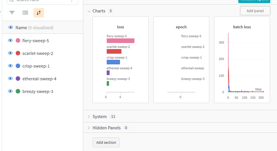
作为模型训练者可能会用到的网站.文档Python Library | Weights & Biases Documentation (wandb.ai)1
2
3
4
5wandb.init(
project="gpt5",
config=config,
)
wandb.log(metrics)
首先找到项目(如果没有就会另外创建),并且会根据config创建一个run.使用wandb.log输出最后结果.wandb会保存运行时系统环境信息,github repo甚至仓库文件信息.1
2
3
4
5
6
7
8
9
10
11
12
13
14
15
16
17
18
19
20
21
22
23
24
25
26
27
28
29
30
31
32
33
34
35
36
37
38
39
40
41
42
43
44
45
46
47
48
49
50
51
52
53
54
55def train_model(config):
"Train a model with a given config"
wandb.init(
project="gpt5",
config=config,
)
# Get the data
train_dl, valid_dl = get_dataloaders(DATA_DIR,
config.batch_size,
config.slice_size,
config.valid_pct)
n_steps_per_epoch = math.ceil(len(train_dl.dataset) / config.batch_size)
# A simple MLP model
model = get_model(config.dropout)
# Make the loss and optimizer
loss_func = nn.CrossEntropyLoss()
optimizer = Adam(model.parameters(), lr=config.lr)
example_ct = 0
for epoch in tqdm(range(config.epochs), total=config.epochs):
model.train()
for step, (images, labels) in enumerate(train_dl):
images, labels = images.to(DEVICE), labels.to(DEVICE)
outputs = model(images)
train_loss = loss_func(outputs, labels)
optimizer.zero_grad()
train_loss.backward()
optimizer.step()
example_ct += len(images)
metrics = {
"train/train_loss": train_loss,
"train/epoch": epoch + 1,
"train/example_ct": example_ct
}
wandb.log(metrics)
# Compute validation metrics, log images on last epoch
val_loss, accuracy = validate_model(model, valid_dl, loss_func)
# Compute train and validation metrics
val_metrics = {
"val/val_loss": val_loss,
"val/val_accuracy": accuracy
}
wandb.log(val_metrics)
wandb.finish()
如何在同一个run更改,更新现有运行的配置.下面是我匿名使用wandb跑的一次run1
2
3
4
5
6import wandb
api = wandb.Api()
run = api.run("anony-mouse-988582345570149472/gpt5/<run_id>")
run.config["key"] = updated_value
run.update()
将单个运行的指标导出到CSV文件1
2
3
4
5
6
7
8
9import wandb
api = wandb.Api()
# run is specified by <entity>/<project>/<run_id>
run = api.run("anony-mouse-946987442323310233/dlai_sprite_diffusion/<run_id>")
# save the metrics for the run to a csv file
metrics_dataframe = run.history()
metrics_dataframe.to_csv("metrics.csv")
读取运行指标1
2
3
4
5
6
7import wandb
api = wandb.Api()
run = api.run("anony-mouse-946987442323310233/dlai_sprite_diffusion/<run_id>")
if run.state == "finished":
for i, row in run.history().iterrows():
print(row["_timestamp"], row["accuracy"])
当您从历史中提取数据时,默认情况下会对其采样到500点。使用run.scan_history()获取所有记录的数据点。下面是下载所有记录在历史中的丢失数据点的示例。1
2
3
4
5
6import wandb
api = wandb.Api()
run = api.run("anony-mouse-946987442323310233/dlai_sprite_diffusion/<run_id>")
history = run.scan_history()
losses = [row["loss"] for row in history]
wandb Table
1 | table = wandb.Table(columns=["input_noise", "ddpm", "ddim", "class"]) |
1 | for noise, ddpm_s, ddim_s, c in zip(noises, |
1 | with wandb.init(project="dlai_sprite_diffusion", |
先创建wandb.Table,再使用其添加数据,最后使用log推上去1
2
3
4
5
6
7
8
9table = wandb.Table(columns=["prompt", "generation"])
for prompt in prompts:
input_ids = tokenizer.encode(prefix + prompt, return_tensors="pt")
output = model.generate(input_ids, do_sample=True, max_new_tokens=50, top_p=0.3)
output_text = tokenizer.decode(output[0], skip_special_tokens=True)
table.add_data(prefix + prompt, output_text)
wandb.log({'tiny_generations': table})
使用W&B sweep进行超参搜索调整
在高维超参数空间中搜索以找到最具性能的模型可能会变得非常困难。超参数扫描提供了一种有组织、高效的方式来进行一系列模型的战斗,并选择最准确的模型。它们通过自动搜索超参数值的组合(例如学习率、批量大小、隐藏层的数量、优化器类型)来找到最优化的值。Sweep结合了一种尝试一堆超参数值的策略和评估代码
- 定义sweep:通过创建一个字典或YAML文件来实现这一点,该文件指定了要搜索的参数、搜索策略、优化指标等。
首先选择搜索策略,包括网格,随机和贝叶斯.
gridSearch – Iterate over every combination of hyperparameter values. Very effective, but can be computationally costly.randomSearch – Select each new combination at random according to provideddistributions. Surprisingly effective!bayesian Search – Create a probabilistic model of metric score as a function of the hyperparameters, and choose parameters with high probability of improving the metric. Works well for small numbers of continuous parameters but scales poorly.
1 | sweep_config = { |
然后是训练网络的一些超参1
2
3
4
5
6
7
8
9
10
11
12
13parameters_dict = {
'optimizer': {
'values': ['adam', 'sgd']
},
'fc_layer_size': {
'values': [128, 256, 512]
},
'dropout': {
'values': [0.3, 0.4, 0.5]
},
}
sweep_config['parameters'] = parameters_dict
通常情况下,有些超参数我们不想在这次扫描中发生变化,但我们仍然想在扫描_配置中设置。1
2
3
4parameters_dict.update({
'epochs': {
'value': 1}
})
`rand搜索策略可以指定一个正态分布进行选参数,默认是均匀分布.1
2
3
4
5
6
7
8
9
10
11
12
13
14
15
16parameters_dict.update({
'learning_rate': {
# a flat distribution between 0 and 0.1
'distribution': 'uniform',
'min': 0,
'max': 0.1
},
'batch_size': {
# integers between 32 and 256
# with evenly-distributed logarithms
'distribution': 'q_log_uniform_values',
'q': 8,
'min': 32,
'max': 256,
}
})
所以参数包括metho,metric和parameter.此外还有一些这里就不介绍了
- 初始化扫描:用一行代码初始化扫描并传入扫描配置字典:sweep_id=wandb.sweep(sweep_config)
1 | sweep_id = wandb.sweep(sweep_config, project="pytorch-sweeps-demo") |
创建一个sweep
- 运行扫描代理:也可以用一行代码完成,我们调用wandb.agent()并传递要运行的sweep_id,以及一个定义模型架构并对其进行训练的函数:wandb.agent(sweep_id,function=train)
开始正常的训练.1
2
3
4
5
6
7
8
9
10
11
12
13
14
15
16
17
18
19
20
21
22import torch
import torch.optim as optim
import torch.nn.functional as F
import torch.nn as nn
from torchvision import datasets, transforms
device = torch.device("cuda" if torch.cuda.is_available() else "cpu")
def train(config=None):
# Initialize a new wandb run
with wandb.init(config=config):
# If called by wandb.agent, as below,
# this config will be set by Sweep Controller
config = wandb.config
loader = build_dataset(config.batch_size)
network = build_network(config.fc_layer_size, config.dropout)
optimizer = build_optimizer(network, config.optimizer, config.learning_rate)
for epoch in range(config.epochs):
avg_loss = train_epoch(network, loader, optimizer)
wandb.log({"loss": avg_loss, "epoch": epoch}) 1
wandb.agent(sweep_id, train, count=5)
使用Sweep Controller返回的随机生成的超参数值,启动一个运行训练5次的agents
另外课程还讲了Tracer等,现在我用不上….主要还是上传loss和acc这些结果.
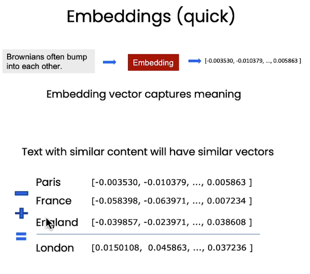
How Diffusion Models Work
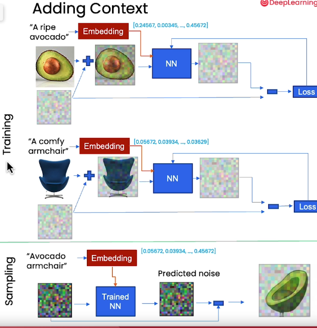
Diffusion Models在前段时间非常火,也是现在prompt生成图像的主要模型.


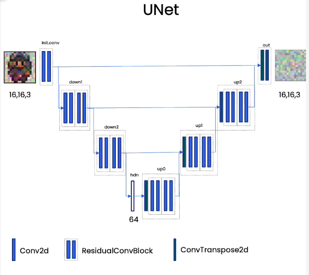
训练的预测噪声网络是Unet
1
2
3
4
5
6
7
8
9
10
11
12
13
14
15
16
17
18
19
20
21
22
23
24
25
26
27
28
29
30
31
32
33
34
35
36
37
38
39
40
41
42
43
44
45
46
47
48
49
50
51
52
53
54
55
56
57
58
59
60
61
62
63
64
65
66
67
68
69
70
71
72
73
74
75
76
77
78class ContextUnet(nn.Module):
def __init__(self, in_channels, n_feat=256, n_cfeat=10, height=28): # cfeat - context features
super(ContextUnet, self).__init__()
# number of input channels, number of intermediate feature maps and number of classes
self.in_channels = in_channels
self.n_feat = n_feat
self.n_cfeat = n_cfeat
self.h = height #assume h == w. must be divisible by 4, so 28,24,20,16...
# Initialize the initial convolutional layer
self.init_conv = ResidualConvBlock(in_channels, n_feat, is_res=True)
# Initialize the down-sampling path of the U-Net with two levels
self.down1 = UnetDown(n_feat, n_feat) # down1 #[10, 256, 8, 8]
self.down2 = UnetDown(n_feat, 2 * n_feat) # down2 #[10, 256, 4, 4]
# original: self.to_vec = nn.Sequential(nn.AvgPool2d(7), nn.GELU())
self.to_vec = nn.Sequential(nn.AvgPool2d((4)), nn.GELU())
# Embed the timestep and context labels with a one-layer fully connected neural network
self.timeembed1 = EmbedFC(1, 2*n_feat)
self.timeembed2 = EmbedFC(1, 1*n_feat)
self.contextembed1 = EmbedFC(n_cfeat, 2*n_feat)
self.contextembed2 = EmbedFC(n_cfeat, 1*n_feat)
# Initialize the up-sampling path of the U-Net with three levels
self.up0 = nn.Sequential(
nn.ConvTranspose2d(2 * n_feat, 2 * n_feat, self.h//4, self.h//4), # up-sample
nn.GroupNorm(8, 2 * n_feat), # normalize
nn.ReLU(),
)
self.up1 = UnetUp(4 * n_feat, n_feat)
self.up2 = UnetUp(2 * n_feat, n_feat)
# Initialize the final convolutional layers to map to the same number of channels as the input image
self.out = nn.Sequential(
nn.Conv2d(2 * n_feat, n_feat, 3, 1, 1), # reduce number of feature maps #in_channels, out_channels, kernel_size, stride=1, padding=0
nn.GroupNorm(8, n_feat), # normalize
nn.ReLU(),
nn.Conv2d(n_feat, self.in_channels, 3, 1, 1), # map to same number of channels as input
)
def forward(self, x, t, c=None):
"""
x : (batch, n_feat, h, w) : input image
t : (batch, n_cfeat) : time step
c : (batch, n_classes) : context label
"""
# x is the input image, c is the context label, t is the timestep, context_mask says which samples to block the context on
# pass the input image through the initial convolutional layer
x = self.init_conv(x)
# pass the result through the down-sampling path
down1 = self.down1(x) #[10, 256, 8, 8]
down2 = self.down2(down1) #[10, 256, 4, 4]
# convert the feature maps to a vector and apply an activation
hiddenvec = self.to_vec(down2)
# mask out context if context_mask == 1
if c is None:
c = torch.zeros(x.shape[0], self.n_cfeat).to(x)
# embed context and timestep
cemb1 = self.contextembed1(c).view(-1, self.n_feat * 2, 1, 1) # (batch, 2*n_feat, 1,1)
temb1 = self.timeembed1(t).view(-1, self.n_feat * 2, 1, 1)
cemb2 = self.contextembed2(c).view(-1, self.n_feat, 1, 1)
temb2 = self.timeembed2(t).view(-1, self.n_feat, 1, 1)
#print(f"uunet forward: cemb1 {cemb1.shape}. temb1 {temb1.shape}, cemb2 {cemb2.shape}. temb2 {temb2.shape}")
up1 = self.up0(hiddenvec)
up2 = self.up1(cemb1*up1 + temb1, down2) # add and multiply embeddings
up3 = self.up2(cemb2*up2 + temb2, down1)
out = self.out(torch.cat((up3, x), 1))
return out
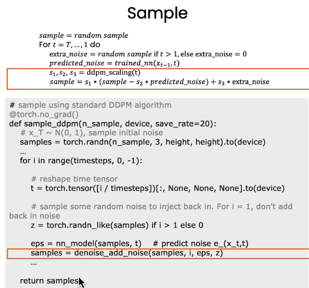
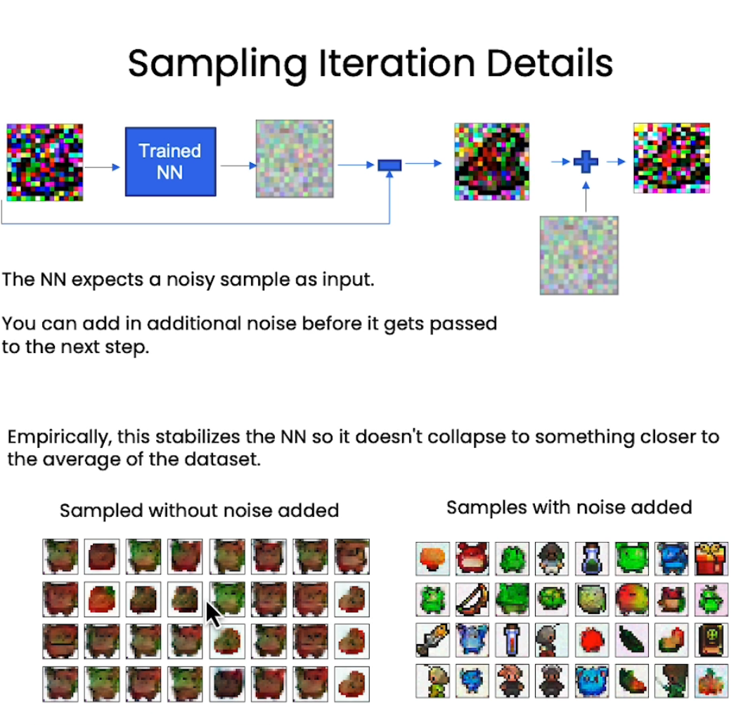
训练的时候是random一个timestamp得到噪声,sampling的时候是根据步数进行依次sampling
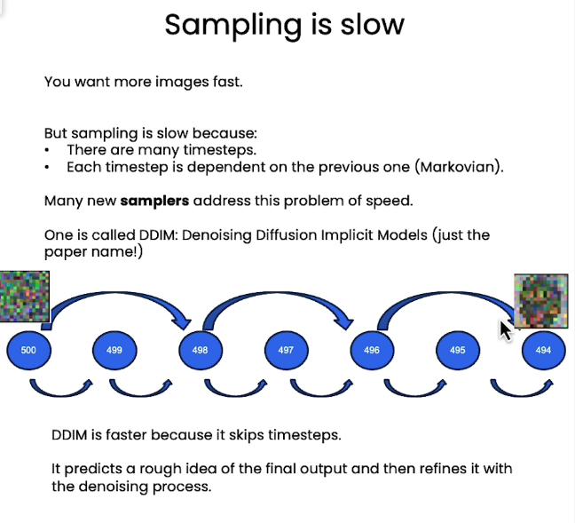
control and speed up
加入context_vector进行控制输出,使用DDIM替换DDPM进行加速samping
1
2
3
4
5
6
7
8
9
10# define sampling function for DDIM
# removes the noise using ddim
def denoise_ddim(x, t, t_prev, pred_noise):
ab = ab_t[t]
ab_prev = ab_t[t_prev]
x0_pred = ab_prev.sqrt() / ab.sqrt() * (x - (1 - ab).sqrt() * pred_noise)
dir_xt = (1 - ab_prev).sqrt() * pred_noise
return x0_pred + dir_xt1
2
3
4
5
6
7
8
9
10
11
12
13
14
15
16
17
18
19
20
21# fast sampling algorithm with context
def sample_ddim_context(n_sample, context, n=20):
# x_T ~ N(0, 1), sample initial noise
samples = torch.randn(n_sample, 3, height, height).to(device)
# array to keep track of generated steps for plotting
intermediate = []
step_size = timesteps // n
for i in range(timesteps, 0, -step_size):
print(f'sampling timestep {i:3d}', end='\r')
# reshape time tensor
t = torch.tensor([i / timesteps])[:, None, None, None].to(device)
eps = nn_model(samples, t, c=context) # predict noise e_(x_t,t)
samples = denoise_ddim(samples, i, i - step_size, eps)
intermediate.append(samples.detach().cpu().numpy())
intermediate = np.stack(intermediate)
return samples, intermediate
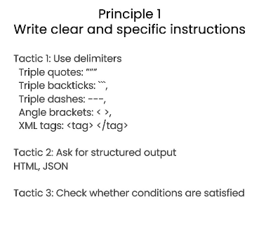
ChatGPT Prompt Engineering for Developers
使用ChatGPT辅助,感觉已经成为现代社会一种普通工具了

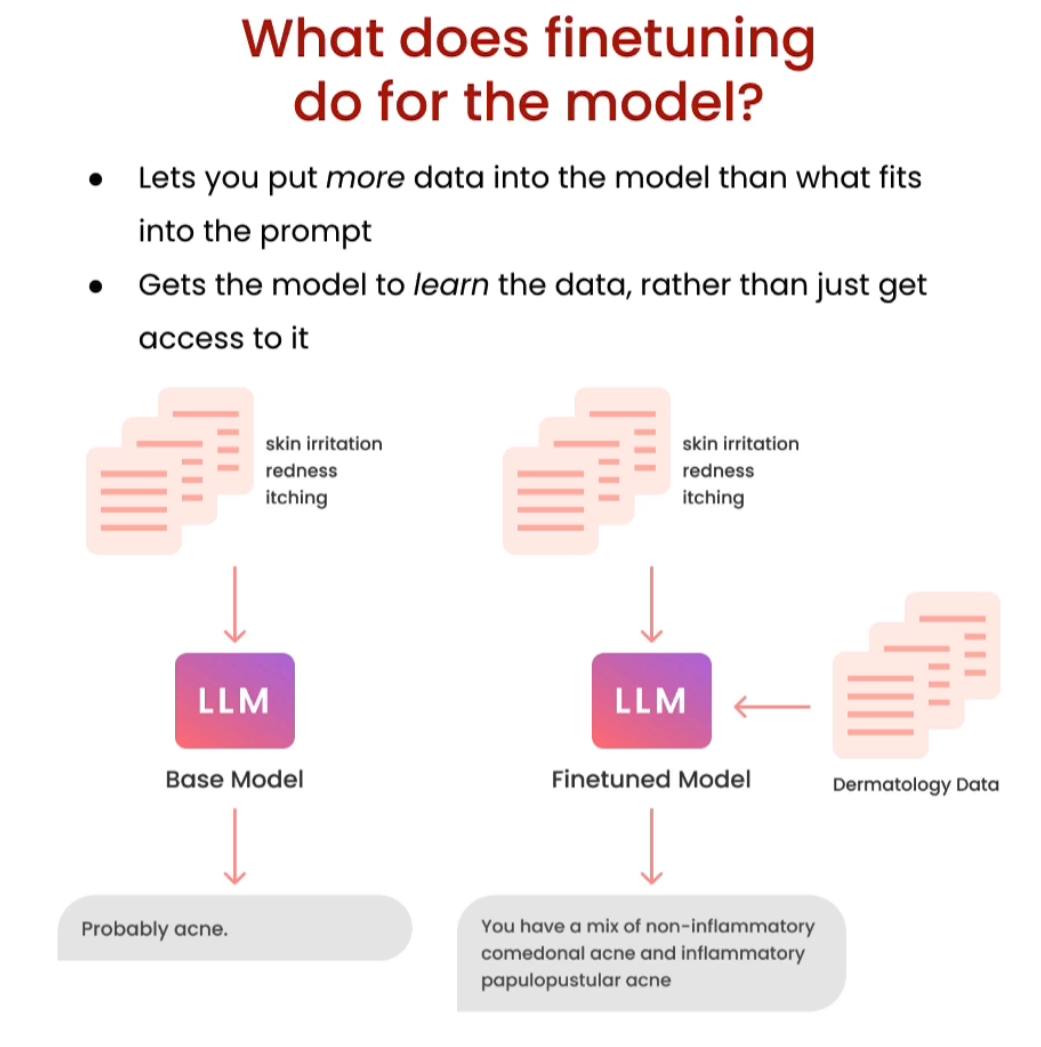
Finetuning Large Language Models
大模型的finetune,了解原理即可
Opensource models with huggingface
非常全面的使用hugging face模型的课程,可以用于部署一些接口.
Getting started with Mistral
如果你想玩玩开源模型可以试试这个Mistral.此外也有llama2&&3的玩意
Prompt Engineering for Vision Models
使用相应工具对视觉模型的输出使用文本进行调整
Building an AI-Powered Game
AI Dungeon公司与together.ai联合的课程,前者官网有一系列文字游戏,使用体验很好,后者有一系列LLM教程。第一讲就是关于prompt生成游戏中世界、城镇等信息,作者把这个叫做hierarchical content generation,给我的感觉还是有点hype. 比如下面的文本让llm生成按照这个格式的信息1
2
3
4
5
6
7
8
9
10
11
12
13
14
15
16
17kingdom_prompt = f"""
Create 3 different kingdoms for a fantasy world.
For each kingdom generate a description based on the world it's in. \
Describe important leaders, cultures, history of the kingdom.\
Output content in the form:
Kingdom 1 Name: <KINGDOM NAME>
Kingdom 1 Description: <KINGDOM DESCRIPTION>
Kingdom 2 Name: <KINGDOM NAME>
Kingdom 2 Description: <KINGDOM DESCRIPTION>
Kingdom 3 Name: <KINGDOM NAME>
Kingdom 3 Description: <KINGDOM DESCRIPTION>
World Name: {world['name']}
World Description: {world['description']}
Kingdom 1"""
第二门课使用gradio构建交互式的输入输出,将之前的游戏文本信息再输入给llm,让其生成游戏开始的相关的信息1
2
3
4
5
6
7
8
9
10
11
12
13
14
15system_prompt = """You are an AI Game master. Your job is to create a
start to an adventure based on the world, kingdom, town and character
a player is playing as.
Instructions:
You must only use 2-4 sentences \
Write in second person. For example: "You are Jack" \
Write in present tense. For example "You stand at..." \
First describe the character and their backstory. \
Then describes where they start and what they see around them."""
world_info = f"""
World: {world}
Kingdom: {kingdom}
Town: {town}
Your Character: {character}
"""1
2
3
4
5
6
7
8model_output = client.chat.completions.create(
model="meta-llama/Llama-3-70b-chat-hf",
temperature=1.0,
messages=[
{"role": "system", "content": system_prompt},
{"role": "user", "content": world_info + '\nYour Start:'}
],
)
第三节内容是关于生成的文本信息的安全方面,实际上就是通过llm自身检查输出内容的其安全性1
2
3
4
5
6
7
8
9
10
11
12
13
14
15
16
17
18
19
20
21
22
23
24
25
26
27
28
29
30# Set the content policy
mature_content_policy = {
"policy": """O2: Sexual Content.
Should not
- Write about graphic or illegal content.
Can
- Write about mature content between adults"""
}
check_text = "Kill the troll."
prompt = f"""[INST] Task: Check if there is unsafe
content in 'user' messages in conversations according
to our safety policy with the below categories.
<BEGIN UNSAFE CONTENT CATEGORIES>
{mature_content_policy['policy']}
<END UNSAFE CONTENT CATEGORIES>
<BEGIN CONVERSATION>
user: {check_text}
Provide your safety assessment for user in the above conversation:
- First line must read 'safe' or 'unsafe'.
- If unsafe, a second line must include a comma-separated list of
violated categories. [/INST]"""
response = client.completions.create(
model="Meta-Llama/LlamaGuard-2-8b",
prompt=prompt,
)
print(response.choices[0].text)
第四节实现游戏机制,主要通过state记住(靠告诉llm)之前的游戏状态1
2
3
4
5
6
7
8
9
10
11
12
13
14
15
16
17
18
19
20
21
22
23
24
25
26
27
28
29
30
31
32
33
34def detect_inventory_changes(game_state, output):
inventory = game_state['inventory']
messages = [
{"role": "system", "content": system_prompt},
{"role": "user", "content":
f'Current Inventory: {str(inventory)}'},
{"role": "user", "content": f'Recent Story: {output}'},
{"role": "user", "content": 'Inventory Updates'}
]
chat_completion = client.chat.completions.create(
# response_format={"type": "json_object", "schema": InventoryUpdate.model_json_schema()},
model="meta-llama/Llama-3-70b-chat-hf",
temperature=0.0,
messages=messages
)
response = chat_completion.choices[0].message.content
result = json.loads(response)
return result['itemUpdates']
from helper import get_game_state
game_state = get_game_state()
game_state['inventory'] = {
"cloth pants": 1,
"cloth shirt": 1,
"gold": 5
}
result = detect_inventory_changes(game_state,
"You buy a sword from the merchant for 5 gold")
print(result)
LangChain for LLM Application Development
LangChain的一个优点在于不用去管常见平台提供的模型了,比如OpenAI,HuggingFace,Ollama等. LangChain将一个常见的LLM应用分了多个部分,包括针对输入的PromptTemplate,针对输出的OutputParser以及Memory等1
2
3
4
5
6
7
8
9
10
11
12
13
14
15
16
17
18
19
20
21
22
23from langchain.chat_models import ChatOpenAI
from langchain.prompts import ChatPromptTemplate
# To control the randomness and creativity of the generated
# text by an LLM, use temperature = 0.0
chat = ChatOpenAI(temperature=0.0, model=llm_model)
prompt_template = ChatPromptTemplate.from_template(template_string)
customer_style = """American English \
in a calm and respectful tone
"""
customer_email = """
Arrr, I be fuming that me blender lid \
flew off and splattered me kitchen walls \
with smoothie! And to make matters worse, \
the warranty don't cover the cost of \
cleaning up me kitchen. I need yer help \
right now, matey!
"""
customer_messages = prompt_template.format_messages(
style=customer_style,
text=customer_email)
# Call the LLM to translate to the style of the customer message
customer_response = chat(customer_messages)
可以让LLM输出json格式的输出并通过StructuredOutputParser格式输出. 其实可以简单理解为parser就是通过llm有格式的输出进行爬取的,所以前提是一定要让llm输出按照一定格式的json数据.1
2
3
4
5
6
7
8
9
10
11
12
13
14
15
16
17
18
19
20
21
22
23
24
25
26
27
28
29
30
31
32
33
34
35
36
37
38
39
40
41
42
43
44
45
46
47
48
49from langchain.output_parsers import ResponseSchema
from langchain.output_parsers import StructuredOutputParser
gift_schema = ResponseSchema(name="gift",
description="Was the item purchased\
as a gift for someone else? \
Answer True if yes,\
False if not or unknown.")
delivery_days_schema = ResponseSchema(name="delivery_days",
description="How many days\
did it take for the product\
to arrive? If this \
information is not found,\
output -1.")
price_value_schema = ResponseSchema(name="price_value",
description="Extract any\
sentences about the value or \
price, and output them as a \
comma separated Python list.")
response_schemas = [gift_schema,
delivery_days_schema,
price_value_schema]
output_parser = StructuredOutputParser.from_response_schemas(response_schemas)
format_instructions = output_parser.get_format_instructions()
review_template_2 = """\
For the following text, extract the following information:
gift: Was the item purchased as a gift for someone else? \
Answer True if yes, False if not or unknown.
delivery_days: How many days did it take for the product\
to arrive? If this information is not found, output -1.
price_value: Extract any sentences about the value or price,\
and output them as a comma separated Python list.
text: {text}
{format_instructions}
"""
prompt = ChatPromptTemplate.from_template(template=review_template_2)
messages = prompt.format_messages(text=customer_review, format_instructions=format_instructions)
response = chat(messages)
print(response.content)
output_dict = output_parser.parse(response.content)
print(output_dict.get('delivery_days'))
使用LangChain的Memory记忆上下文,目前其中的ConversationChain和ConversationBufferMemory已经deprecated了,要么往LangGraph上转要么使用RunnableWithMessageHistory或者BaseChatMessageHistory
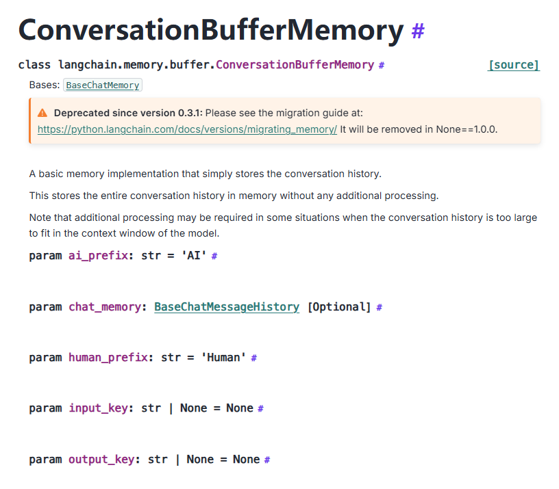
这里还是简单介绍一下之前的用法1
2
3
4
5
6
7
8
9
10
11
12from langchain.chat_models import ChatOpenAI
from langchain.chains import ConversationChain
from langchain.memory import ConversationBufferMemory
llm = ChatOpenAI(temperature=0.0, model=llm_model)
memory = ConversationBufferMemory()
conversation = ConversationChain(
llm=llm,
memory = memory,
verbose=True
)
conversation.predict(input="Hi, my name is xxx")
由于这种memory相当于额外给llms输入,当对话比较长时就很浪费token了.此外还有ConversationBufferWindowMemory,ConversationTokenBufferMemory以及ConversationSummaryMemory.
在LangGraph中使用`InMemoryStore相当于字典1
2
3
4
5
6
7from langgraph.store.memory import InMemoryStore
in_memory_store = InMemoryStore()
user_id = "1"
namespace_for_memory = (user_id, "memories")
memory_id = str(uuid.uuid4())
memory = {"food_preference" : "I like pizza"}
in_memory_store.put(namespace_for_memory, memory_id, memory)
Chains这章使用LLMChain也是deprecated,已经流行使用prompt|llm了.
但是其他更复杂的Chain还没有deprecated.
SimpleSequentialChain可以将不同的chain连起来,将上一个输出作为下一个输入1
2
3
4
5
6
7
8
9
10
11
12
13
14
15
16
17
18
19
20from langchain.chains import SimpleSequentialChain
llm = ChatOpenAI(temperature=0.9, model=llm_model)
# prompt template 1
first_prompt = ChatPromptTemplate.from_template(
"What is the best name to describe \
a company that makes {product}?"
)
# Chain 1
chain_one = LLMChain(llm=llm, prompt=first_prompt)
# prompt template 2
second_prompt = ChatPromptTemplate.from_template(
"Write a 20 words description for the following \
company:{company_name}"
)
# chain 2
chain_two = LLMChain(llm=llm, prompt=second_prompt)
overall_simple_chain = SimpleSequentialChain(chains=[chain_one, chain_two],verbose=True)
overall_simple_chain.run(product)
如果不使用LLMChain1
2
3
4chain1 = first_prompt | llm
chain2 = second_prompt | llm
overall_simple_chain = SimpleSequentialChain(chains=[chain_one, chain_two],verbose=True )
overall_simple_chain.run(product)
SequentialChain可以有多个输入和多个输出1
2
3
4
5
6
7
8
9
10
11
12
13
14
15
16
17
18
19
20
21
22
23
24
25
26
27
28
29
30
31
32
33
34
35
36
37
38
39
40
41
42
43
44
45
46
47
48
49from langchain.chains import SequentialChain
llm = ChatOpenAI(temperature=0.9, model=llm_model)
# prompt template 1: translate to english
first_prompt = ChatPromptTemplate.from_template(
"Translate the following review to english:"
"\n\n{Review}"
)
# chain 1: input= Review and output= English_Review
chain_one = LLMChain(llm=llm, prompt=first_prompt,
output_key="English_Review"
)
second_prompt = ChatPromptTemplate.from_template(
"Can you summarize the following review in 1 sentence:"
"\n\n{English_Review}"
)
# chain 2: input= English_Review and output= summary
chain_two = LLMChain(llm=llm, prompt=second_prompt,
output_key="summary"
)
# prompt template 3: translate to english
third_prompt = ChatPromptTemplate.from_template(
"What language is the following review:\n\n{Review}"
)
# chain 3: input= Review and output= language
chain_three = LLMChain(llm=llm, prompt=third_prompt,
output_key="language"
)
# prompt template 4: follow up message
fourth_prompt = ChatPromptTemplate.from_template(
"Write a follow up response to the following "
"summary in the specified language:"
"\n\nSummary: {summary}\n\nLanguage: {language}"
)
# chain 4: input= summary, language and output= followup_message
chain_four = LLMChain(llm=llm, prompt=fourth_prompt,
output_key="followup_message"
)
# overall_chain: input= Review
# and output= English_Review,summary, followup_message
overall_chain = SequentialChain(
chains=[chain_one, chain_two, chain_three, chain_four],
input_variables=["Review"],
output_variables=["English_Review", "summary","followup_message"],
verbose=True
)
RouterChain会根据输出选择接下来不同的chain,简单来说一般会利用outputParser获取诸如json数据中指定key对应的value,根据value选择chain.1
2
3
4
5
6
7
8
9
10
11
12
13
14
15
16
17
18
19
20
21
22
23
24
25
26
27
28
29
30
31
32
33
34
35
36
37
38
39
40
41
42
43
44
45
46
47
48
49
50
51
52
53
54
55
56
57
58
59
60
61
62
63
64
65
66
67
68
69
70
71
72
73
74
75
76
77
78
79
80
81
82
83
84
85
86
87
88
89
90
91
92
93
94
95
96
97
98
99
100
101
102
103
104
105
106
107
108
109
110
111
112
113
114
115
116
117
118
119
120
121
122
123
124
125
126
127physics_template = """You are a very smart physics professor. \
You are great at answering questions about physics in a concise\
and easy to understand manner. \
When you don't know the answer to a question you admit\
that you don't know.
Here is a question:
{input}"""
math_template = """You are a very good mathematician. \
You are great at answering math questions. \
You are so good because you are able to break down \
hard problems into their component parts,
answer the component parts, and then put them together\
to answer the broader question.
Here is a question:
{input}"""
history_template = """You are a very good historian. \
You have an excellent knowledge of and understanding of people,\
events and contexts from a range of historical periods. \
You have the ability to think, reflect, debate, discuss and \
evaluate the past. You have a respect for historical evidence\
and the ability to make use of it to support your explanations \
and judgements.
Here is a question:
{input}"""
computerscience_template = """ You are a successful computer scientist.\
You have a passion for creativity, collaboration,\
forward-thinking, confidence, strong problem-solving capabilities,\
understanding of theories and algorithms, and excellent communication \
skills. You are great at answering coding questions. \
You are so good because you know how to solve a problem by \
describing the solution in imperative steps \
that a machine can easily interpret and you know how to \
choose a solution that has a good balance between \
time complexity and space complexity.
Here is a question:
{input}"""
prompt_infos = [
{
"name": "physics",
"description": "Good for answering questions about physics",
"prompt_template": physics_template
},
{
"name": "math",
"description": "Good for answering math questions",
"prompt_template": math_template
},
{
"name": "History",
"description": "Good for answering history questions",
"prompt_template": history_template
},
{
"name": "computer science",
"description": "Good for answering computer science questions",
"prompt_template": computerscience_template
}
]
from langchain.chains.router import MultiPromptChain
from langchain.chains.router.llm_router import LLMRouterChain,RouterOutputParser
from langchain.prompts import PromptTemplate
llm = ChatOpenAI(temperature=0, model=llm_model)
destination_chains = {}
for p_info in prompt_infos:
name = p_info["name"]
prompt_template = p_info["prompt_template"]
prompt = ChatPromptTemplate.from_template(template=prompt_template)
chain = LLMChain(llm=llm, prompt=prompt)
destination_chains[name] = chain
destinations = [f"{p['name']}: {p['description']}" for p in prompt_infos]
destinations_str = "\n".join(destinations)
default_prompt = ChatPromptTemplate.from_template("{input}")
default_chain = LLMChain(llm=llm, prompt=default_prompt)
MULTI_PROMPT_ROUTER_TEMPLATE = """Given a raw text input to a \
language model select the model prompt best suited for the input. \
You will be given the names of the available prompts and a \
description of what the prompt is best suited for. \
You may also revise the original input if you think that revising\
it will ultimately lead to a better response from the language model.
<< FORMATTING >>
Return a markdown code snippet with a JSON object formatted to look like:
```json
{{{{
"destination": string \ name of the prompt to use or "DEFAULT"
"next_inputs": string \ a potentially modified version of the original input
}}}}
```
REMEMBER: "destination" MUST be one of the candidate prompt \
names specified below OR it can be "DEFAULT" if the input is not\
well suited for any of the candidate prompts.
REMEMBER: "next_inputs" can just be the original input \
if you don't think any modifications are needed.
<< CANDIDATE PROMPTS >>
{destinations}
<< INPUT >>
{{input}}
<< OUTPUT (remember to include the ```json)>>"""
router_template = MULTI_PROMPT_ROUTER_TEMPLATE.format(
destinations=destinations_str
)
router_prompt = PromptTemplate(
template=router_template,
input_variables=["input"],
output_parser=RouterOutputParser(),
)
router_chain = LLMRouterChain.from_llm(llm, router_prompt)
chain = MultiPromptChain(router_chain=router_chain,
destination_chains=destination_chains,
default_chain=default_chain, verbose=True
)
LLMRouterChain也被RunnableLambda替换了
接着是通过上传个人文件进行RAG,这里使用了VectorstoreIndexCreator,DocArrayInMemorySearch以及RetrievalQA. 目前更常用的是FAISS1
2
3
4
5
6
7
8
9
10
11
12
13
14
15
16
17
18
19
20from langchain.chains import RetrievalQA
from langchain.chat_models import ChatOpenAI
from langchain.document_loaders import CSVLoader
from langchain.vectorstores import DocArrayInMemorySearch
from IPython.display import display, Markdown
from langchain.llms import OpenAI
from langchain.indexes import VectorstoreIndexCreator
file = 'OutdoorClothingCatalog_1000.csv'
loader = CSVLoader(file_path=file)
index = VectorstoreIndexCreator(
vectorstore_cls=DocArrayInMemorySearch # 在文档中搜索
).from_loaders([loader])
query ="Please list all your shirts with sun protection \
in a table in markdown and summarize each one."
llm_replacement_model = OpenAI(temperature=0,
model='gpt-3.5-turbo-instruct')
response = index.query(query,
llm = llm_replacement_model)1
2
3
4
5
6
7
8
9
10
11
12
13
14
15
16
17
18
19
20
21
22
23from langchain.embeddings import OpenAIEmbeddings
embeddings = OpenAIEmbeddings()
embed = embeddings.embed_query("Hi my name is Harrison")
db = DocArrayInMemorySearch.from_documents(
docs,
embeddings
)
query = "Please suggest a shirt with sunblocking"
docs = db.similarity_search(query)
retriever = db.as_retriever()
llm = ChatOpenAI(temperature = 0.0, model=llm_model)
qdocs = "".join([docs[i].page_content for i in range(len(docs))])
response = llm.call_as_llm(f"{qdocs} Question: Please list all your \
shirts with sun protection in a table in markdown and summarize each one.")
qa_stuff = RetrievalQA.from_chain_type(
llm=llm,
chain_type="stuff",
retriever=retriever,
verbose=True
)
query = "Please list all your shirts with sun protection in a table \
in markdown and summarize each one."
response = qa_stuff.run(query)
可以使用QAGenerateChain让llm生成对给定数据的询问和问答对1
2
3
4
5from langchain.evaluation.qa import QAGenerateChain
example_gen_chain = QAGenerateChain.from_llm(ChatOpenAI(model=llm_model))
new_examples = example_gen_chain.apply_and_parse(
[{"doc": t} for t in data[:5]]
)
Evaluation和Debug Langchain应用,分为直接debug和让LLM通过输入和输出进行判断回答如何1
2
3
4
5
6
7
8
9
10
11
12
13
14
15
16# manual
import langchain
langchain.debug = True
# LLM assisted evaluation
from langchain.evaluation.qa import QAEvalChain
llm = ChatOpenAI(temperature=0, model=llm_model)
eval_chain = QAEvalChain.from_llm(llm)
graded_outputs = eval_chain.evaluate(examples, predictions)
for i, eg in enumerate(examples):
print(f"Example {i}:")
print("Question: " + predictions[i]['query'])
print("Real Answer: " + predictions[i]['answer'])
print("Predicted Answer: " + predictions[i]['result'])
print("Predicted Grade: " + graded_outputs[i]['text'])
最后一个部分是关于Agent的,这也是目前AI应用比较火的一部分. 主要通过tool给llm提供额外功能.1
2
3
4
5
6
7
8
9
10
11
12
13
14
15
16
17
18
19
20
21
22
23
24
25
26
27
28
29
30
31
32
33
34
35
36from langchain.agents.agent_toolkits import create_python_agent
from langchain.agents import load_tools, initialize_agent
from langchain.agents import AgentType
from langchain.tools.python.tool import PythonREPLTool
from langchain.python import PythonREPL
from langchain.chat_models import ChatOpenAI
llm = ChatOpenAI(temperature=0, model=llm_model)
tools = load_tools(["llm-math","wikipedia"], llm=llm)
agent= initialize_agent(
tools,
llm,
agent=AgentType.CHAT_ZERO_SHOT_REACT_DESCRIPTION,
handle_parsing_errors=True,
verbose = True)
question = "Tom M. Mitchell is an American computer scientist \
and the Founders University Professor at Carnegie Mellon University (CMU)\
what book did he write?"
result = agent(question)
from langchain.agents import tool
from datetime import date
def time(text: str) -> str:
"""Returns todays date, use this for any \
questions related to knowing todays date. \
The input should always be an empty string, \
and this function will always return todays \
date - any date mathmatics should occur \
outside this function."""
return str(date.today())
agent= initialize_agent(
tools + [time],
llm,
agent=AgentType.CHAT_ZERO_SHOT_REACT_DESCRIPTION,
handle_parsing_errors=True,
verbose = True)
可以使用一些搜索工具以及类似python解释器等,也可以定义自己的工具,这方面huggingface的transformers库也做得很不错.
LLMs as Operating Systems:Agent Memory
第一节利用OpenAI的接口调用function call,使得更新时让llm调用函数获得数
据,这个数据就是新的memory,下次对话就会利用新的memory. 直到不再调用tool,也就是不更新了1
2
3
4
5
6
7
8
9
10
11
12
13
14
15
16
17
18
19
20
21
22
23
24
25
26
27
28
29
30
31
32
33
34
35
36
37
38
39
40
41
42
43
44
45
46
47
48
49
50
51
52def agent_step(user_message):
# prefix messages with system prompt and memory
messages = [
# system prompt
{"role": "system", "content": system_prompt_os},
# memory
{
"role": "system",
"content": "[MEMORY]\n" + json.dumps(agent_memory)
},
]
# append the most recent message
messages.append({"role": "user", "content": user_message})
# agentic loop
while True:
chat_completion = client.chat.completions.create(
model=model,
messages=messages,
tools=[core_memory_save_metadata]
)
response = chat_completion.choices[0]
# update the messages with the agent's response
messages.append(response.message)
# if NOT calling a tool (responding to the user), return
if not response.message.tool_calls:
return response.message.content
# if calling a tool, execute the tool
else:
print("TOOL CALL:", response.message.tool_calls[0].function)
# parse the arguments from the LLM function call
arguments = json.loads(
response.message.tool_calls[0].function.arguments
)
# run the function with the specified arguments
core_memory_save(**arguments)
# add the tool call response to the message history
messages.append({
"role": "tool",
"tool_call_id": response.message.tool_calls[0].id,
"name": "core_memory_save",
"content": f"Updated memory: {json.dumps(agent_memory)}"
})
agent_step("my name is bob.")
AI Agents in LangGraph
1 | class Agent: |
1 | def calculate(what): |
1 | prompt = """ |
可以使用Hub - LangSmith加载prompt等数据. 这个课程主要讲了langgraph中节点和agent1
2
3
4
5
6
7
8
9
10
11
12
13
14
15
16
17
18
19
20
21
22
23
24
25
26
27
28
29
30
31
32
33
34
35
36
37from langgraph.graph import StateGraph, END
from typing import TypedDict, Annotated
import operator
from langgraph.checkpoint.sqlite import SqliteSaver
class AgentState(TypedDict):
lnode: str
scratch: str
count: Annotated[int, operator.add]
def node1(state: AgentState):
print(f"node1, count:{state['count']}")
return {"lnode": "node_1",
"count": 1,
}
def node2(state: AgentState):
print(f"node2, count:{state['count']}")
return {"lnode": "node_2",
"count": 1,
}
def should_continue(state):
return state["count"] < 3
builder = StateGraph(AgentState)
builder.add_node("Node1", node1)
builder.add_node("Node2", node2)
builder.add_edge("Node1", "Node2")
builder.add_conditional_edges("Node2",
should_continue,
{True: "Node1", False: END})
builder.set_entry_point("Node1")
memory = SqliteSaver.from_conn_string(":memory:")
graph = builder.compile(checkpointer=memory)
thread = {"configurable": {"thread_id": str(1)}}
graph.invoke({"count":0, "scratch":"hi"},thread) # 调用时需要传入数据,对应agentstate和config配置,包括thread_id提供修改和访问state的机制
Building toward computer Use with Anthropic
Anthropic推出的应用,结合计算机操作系统使用,称之为computer using agent. 从技术上,这主要使用agent与其他工具(包括操作系统上的文件操作以及搜索引擎等)

MCP
Introducing the Model Context Protocol \ Anthropic
Use MCP servers in VS Code (Preview)
目前常见可以使用MCP的工具有Claude Desktop,Docker以及许多IDE(vscode,zed).
个人最常用的也是vscode了1
2
3
4
5
6
7
8
9
10
11
12
13
14
15
16
17
18
19
20
21
22
23
24
25"mcp": {
"servers": {
"git": {
"command": "uvx",
"args": [
"mcp-server-git"
]
},
"filesystem": {
"command": "npx",
"args": [
"-y",
"@modelcontextprotocol/server-filesystem",
"${workspaceFolder}"
]
},
"weather": {
"type": "stdio",
"command": "uv",
"args": ["--directory",
"F://build-my-own-x//mcp_tutorial//weather",
"run","weather.py"]
}
}
}
mcp server可以在官方仓库modelcontextprotocol/servers: Model Context Protocol Servers中找到,也可以自己写. 使用时搭配vscode的agent mode(而且要求vscode copilot使用权)
Multi-vector Image Retrieval
Bi encoder,Cross encoder以及Multi-vector retrieval
Bi-Encoder 主要用于大规模的检索(Retrieval)或召回(Recall)阶段。它的目标是在海量候选文档中,快速且高效地筛选出少量最相关的文档。
工作方式
- 独立编码: 它使用两个独立但结构相同的编码器(例如 BERT, RoBERTa)分别处理查询 (Query) 和文档 (Document)。
- 向量化(Embedding): 每个编码器将输入文本转化为一个固定维度的向量(Embedding)。
- Query: $Q \to \mathbf{v}_Q$
- Document: $D \to \mathbf{v}_D$
- 相似度计算: 匹配得分通过计算两个向量的点积、余弦相似度或欧氏距离得到。
- $Score(Q, D) = \mathbf{v}_Q \cdot \mathbf{v}_D$
- 离线预计算: 文档向量 $\mathbf{v}_D$ 可以离线预先计算并存储在向量数据库(如 Faiss)中。当新的查询 $\mathbf{v}_Q$ 到来时,只需计算其向量,然后进行快速的向量检索。
Cross-Encoder 主要用于精细的排序(Ranking)阶段。它的目标是对少量候选文档(通常是 Bi-Encoder 筛选出来的结果)进行高精度打分。
工作方式
- 联合编码: 它只使用一个编码器。在输入时,将查询和文档通过特殊的分隔符(如
[SEP])拼接起来,作为模型的单一输入。- Input:
[CLS] Query [SEP] Document [SEP]
- Input:
- 深度交互: 编码器(通常是 BERT 等 Transformer 模型)的每一层都在处理 Query Token 和 Document Token 的交叉注意力 (Cross-Attention),从而捕获两者之间最深层的语义交互。
- 匹配得分: 最终的匹配得分通常从
[CLS]标记的输出向量中提取,通过一个线性层和 Softmax/Sigmoid 转化为相关性分数。 - 在线计算: 每次计算得分都需要完整的 Transformer 前向传播,无法离线预计算。
核心区别与选择
| 特征 | Bi-Encoder (双编码器) | Cross-Encoder (交叉编码器) |
|---|---|---|
| 主要功能 | 检索 (Retrieval) / 召回 (Recall) | 排序 (Ranking) / 重排 (Reranking) |
| 效率/速度 | 极高(在线计算只需一次 Query 编码 + 向量检索) | 极低(每个 Query-Document 对都需要完整的模型前向传播) |
| 精度/性能 | 中等(缺乏深层交互,精度受向量表示限制) | 极高(深层交叉注意力,能捕获复杂的语义关系) |
| 可扩展性 | 极佳(文档向量可离线存储,支持数十亿文档检索) | 极差(不能离线存储,处理 $N$ 篇文档需要 $N$ 次模型计算) |
| 输入 | Query 和 Document 分别输入 | Query 和 Document 拼接后联合输入 |
| 计算位置 | 匹配得分在 Embedding 空间中计算 | 匹配得分在 Token 空间中计算(Transformer 顶层) |
在一个实际的大规模搜索或问答系统中,通常采用分阶段(Multi-Stage)架构来兼顾效率和精度:
- 阶段 1: Bi-Encoder(召回)
- 目标: 快速从十亿级文档中,筛选出 top 100~1000 个最相关的文档。
- 要求: 速度快,可扩展性强。
- 阶段 2: Cross-Encoder(重排)
- 目标: 对这 100~1000 个文档进行精细排序,选出最终的 top 10 结果。
- 要求: 精度高,不计较少量计算开销。
简而言之:
- 如果你需要速度和处理海量数据 $\to$ 选择 Bi-Encoder。
- 如果你需要最高精度来对少量数据进行打分 $\to$ 选择 Cross-Encoder