最近OpenAI的Sora模型又大火了一把,据说背后的技术是transformer+diffusion.之前我也大致介绍过stable diffusion的过程,这里我再稍微详细介绍一下经典的扩散模型以及改进之后的DDIM.其中我也有很多不太明白的,只有结合代码理解了.

相关论文[2006.11239] Denoising Diffusion Probabilistic Models (arxiv.org)与[2010.02502] Denoising Diffusion Implicit Models (arxiv.org),2112.10752.pdf (arxiv.org)

Stable Diffusion is a latent text-to-image diffusion model.

已经提出了几种基于扩散的生成模型，其下有类似的想法，包括扩散概率模型、噪声条件评分网络和去噪扩散概率模型。现在常说的基于扩散的生成模型通常指的后者DDPM或者改进的DDIM.

前向扩散过程

$$q(\mathbf{x}_t|\mathbf{x}_{t-1})=\mathcal{N}(\mathbf{x}_t;\sqrt{1-\beta_t}\mathbf{x}_{t-1},\beta_t\mathbf{I})\quad q(\mathbf{x}_{1:T}|\mathbf{x}_0)=\prod_{t=1}^Tq(\mathbf{x}_t|\mathbf{x}_{t-1})$$

所谓的扩散就是给图片(或者是特征,比如stable diffusion就是在所谓latent空间上进行扩散的)加噪声,所加的噪声按照一定分布.

前向过程为一个马尔科夫链,使用重参数化(在VAE中也有),可以表示为

$$\begin{aligned}\mathbf{x}_t&=\sqrt{\alpha_t}\mathbf{x}_{t-1}+\sqrt{1-\alpha_t}\boldsymbol{\epsilon}_{t-1}&&\text{;where }\boldsymbol{\epsilon}_{t-1},\boldsymbol{\epsilon}_{t-2},\cdots\sim\mathcal{N}(\boldsymbol{0},\mathbf{I})\\&=\sqrt{\alpha_t\alpha_{t-1}}\mathbf{x}_{t-2}+\sqrt{1-\alpha_t\alpha_{t-1}}\boldsymbol{\bar{\epsilon}}_{t-2}&&\text{;where }\boldsymbol{\bar{\boldsymbol{\epsilon}}}_{t-2}\text{ merges two Gaussians }(*).\\&=\ldots\\&=\sqrt{\alpha}_t\mathbf{x}_0+\sqrt{1-\bar{\alpha}_t}\boldsymbol{\epsilon}&&\text{j}\\q(\mathbf{x}_t|\mathbf{x}_0)&=\mathcal{N}(\mathbf{x}_t;\sqrt{\alpha}_t\mathbf{x}_0,(1-\bar{\alpha}_t)\mathbf{I})\end{aligned}$$

其中α=1-β.$\bar{\alpha}{t}=\prod{i=1}^{t}\alpha_{i}$,β是从0到1中间的采样值,比如0.01,0.02..

1 2 3 4 5 6 7 8 9 10 11 12 13 14 15 16 17 18 19 20 21 22 23 24 25 26 27 28 29 30 31 32 33 34 35 36 37 38 39 40 41

import torch.nn.functional as F def linear_beta_schedule(timesteps, start=0.0001, end=0.02): return torch.linspace(start, end, timesteps) def get_index_from_list(vals, t, x_shape): """ Returns a specific index t of a passed list of values vals while considering the batch dimension. """ batch_size = t.shape[0] out = vals.gather(-1, t.cpu()) return out.reshape(batch_size, *((1,) * (len(x_shape) - 1))).to(t.device) def forward_diffusion_sample(x_0, t, device="cpu"): """ Takes an image and a timestep as input and returns the noisy version of it """ noise = torch.randn_like(x_0) sqrt_alphas_cumprod_t = get_index_from_list(sqrt_alphas_cumprod, t, x_0.shape) sqrt_one_minus_alphas_cumprod_t = get_index_from_list( sqrt_one_minus_alphas_cumprod, t, x_0.shape ) # mean + variance return sqrt_alphas_cumprod_t.to(device) * x_0.to(device) \ + sqrt_one_minus_alphas_cumprod_t.to(device) * noise.to(device), noise.to(device) # Define beta schedule T = 300 betas = linear_beta_schedule(timesteps=T) # Pre-calculate different terms for closed form alphas = 1. - betas alphas_cumprod = torch.cumprod(alphas, axis=0) alphas_cumprod_prev = F.pad(alphas_cumprod[:-1], (1, 0), value=1.0) sqrt_recip_alphas = torch.sqrt(1.0 / alphas) sqrt_alphas_cumprod = torch.sqrt(alphas_cumprod) sqrt_one_minus_alphas_cumprod = torch.sqrt(1. - alphas_cumprod) posterior_variance = betas * (1. - alphas_cumprod_prev) / (1. - alphas_cumprod)

加噪声的schedule有多种

1 2 3 4 5 6 7 8 9 10 11 12 13 14 15 16 17 18 19 20 21 22 23 24 25 26 27

def cosine_beta_schedule(timesteps, s=0.008): """ cosine schedule as proposed in https://arxiv.org/abs/2102.09672 """ steps = timesteps + 1 x = torch.linspace(0, timesteps, steps) alphas_cumprod = torch.cos(((x / timesteps) + s) / (1 + s) * torch.pi * 0.5) ** 2 alphas_cumprod = alphas_cumprod / alphas_cumprod[0] betas = 1 - (alphas_cumprod[1:] / alphas_cumprod[:-1]) return torch.clip(betas, 0.0001, 0.9999) def linear_beta_schedule(timesteps): beta_start = 0.0001 beta_end = 0.02 return torch.linspace(beta_start, beta_end, timesteps) def quadratic_beta_schedule(timesteps): beta_start = 0.0001 beta_end = 0.02 return torch.linspace(beta_start**0.5, beta_end**0.5, timesteps) ** 2 def sigmoid_beta_schedule(timesteps): beta_start = 0.0001 beta_end = 0.02 betas = torch.linspace(-6, 6, timesteps) return torch.sigmoid(betas) * (beta_end - beta_start) + beta_start

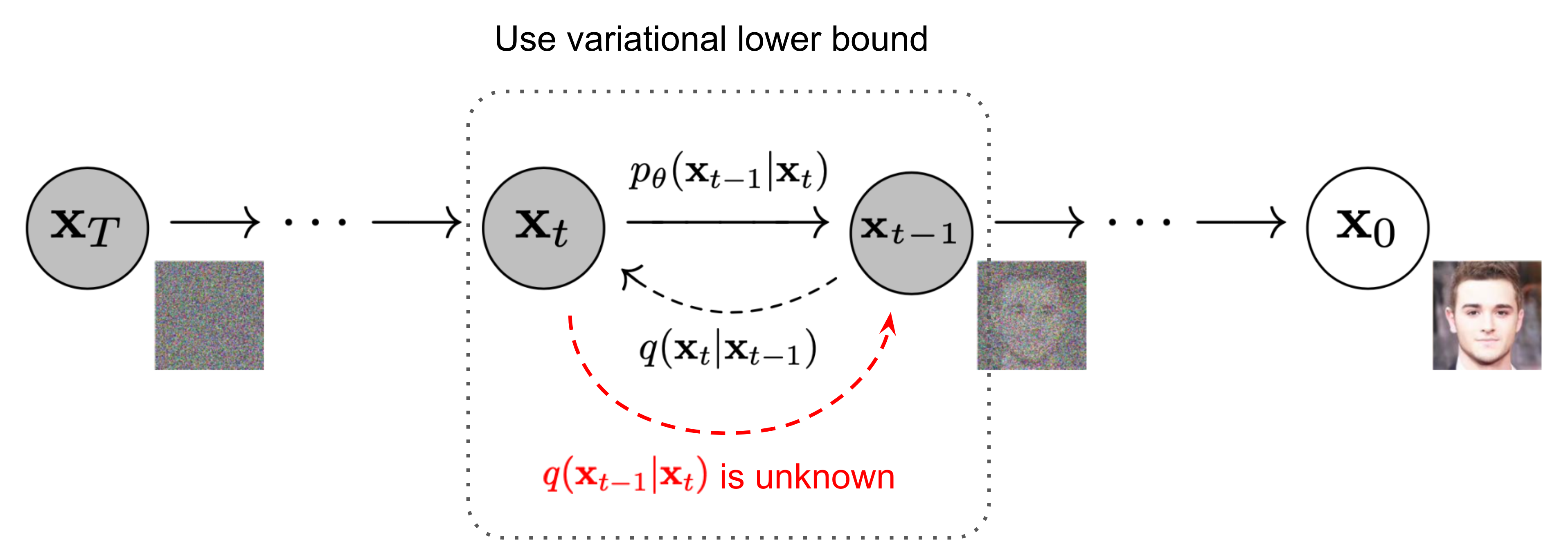
反向扩散过程

如果能将上述过程反向,就能从高斯噪声图像得到一整图像了.也就是需要知道$q(\mathbf{x}{t-1}|\mathbf{x}{t})$,这跟贝叶斯有点关系,可以使用神经网络近似这个条件概率,以便运行反向扩散过程.

$$p_\theta(\mathbf{x}_{0:T})=p(\mathbf{x}_T)\prod_{t=1}^Tp_\theta(\mathbf{x}_{t-1}|\mathbf{x}_t)\quad p_\theta(\mathbf{x}_{t-1}|\mathbf{x}_t)=\mathcal{N}(\mathbf{x}_{t-1};\boldsymbol{\mu}_\theta(\mathbf{x}_t,t),\boldsymbol{\Sigma}_\theta(\mathbf{x}_t,t))$$

假设反向也是高斯,可以有条件概率

$$q(\mathbf{x}_{t-1}|\mathbf{x}_t,\mathbf{x}_0)=\mathcal{N}(\mathbf{x}_{t-1};\tilde{\boldsymbol{\mu}}(\mathbf{x}_t,\mathbf{x}_0),\color{red}{\tilde{\boldsymbol{\beta}}_t}\mathbf{I})$$

使用贝叶斯

$$\begin{aligned} q(\mathbf{x}_{t-1}|\mathbf{x}_t,\mathbf{x}_0)& =q(\mathbf{x}_t|\mathbf{x}_{t-1},\mathbf{x}_0)\frac{q(\mathbf{x}_{t-1}|\mathbf{x}_0)}{q(\mathbf{x}_t|\mathbf{x}_0)} \\ &\propto\exp\left(-\frac12(\frac{(\mathbf{x}_t-\sqrt{\alpha_t}\mathbf{x}_{t-1})^2}{\beta_t}+\frac{(\mathbf{x}_{t-1}-\sqrt{\bar{\alpha}_{t-1}}\mathbf{x}_0)^2}{1-\bar{\alpha}_{t-1}}-\frac{(\mathbf{x}_t-\sqrt{\bar{\alpha}_t}\mathbf{x}_0)^2}{1-\bar{\alpha}_t})\right) \\ &=\exp\left(-\frac12(\frac{\mathbf{x}_t^2-2\sqrt{\alpha_t}\mathbf{x}_t\mathbf{x}_{t-1}+\alpha_t\mathbf{x}_{t-1}^2}{\beta_t}+\frac{\mathbf{x}_{t-1}^2-2\sqrt{\bar{\alpha}_{t-1}}\mathbf{x}_0\mathbf{x}_{t-1}+\bar{\alpha}_{t-1}\mathbf{x}_0^2}{1-\bar{\alpha}_{t-1}}-\frac{(\mathbf{x}_t-\sqrt{\bar{\alpha}_t}\mathbf{x}_0)^2}{1-\bar{\alpha}_t})\right) \\ &\left.=\exp\left(-\frac12(\color{red}{(\frac{\alpha_t}{\beta_t}+\frac1{1-\bar{\alpha}_{t-1}})x_{t-1}^2-(\frac{2\sqrt{\alpha_t}}{\beta_t}x_t+\frac{2\sqrt{\bar{\alpha}_{t-1}}}{1-\bar{\alpha}_{t-1}}x_0)x_{t-1}+C(\mathbf{x}_t,\mathbf{x}_0)}\right)\right) \end{aligned}$$

根据一堆公式计算(这不是我擅长的),得到均值和方差.

$$\begin{aligned} \tilde{\beta}_{t}& =1/(\frac{\alpha_t}{\beta_t}+\frac{1}{1-\bar{\alpha}_{t-1}})=1/(\frac{\alpha_t-\bar{\alpha}_t+\beta_t}{\beta_t(1-\bar{\alpha}_{t-1})})=\frac{1-\bar{\alpha}_{t-1}}{1-\bar{\alpha}_t}\cdot\beta_t \\ \tilde{\boldsymbol{\mu}}_t(\mathbf{x}_t,\mathbf{x}_0)& =(\frac{\sqrt{\alpha_t}}{\beta_t}\mathbf{x}_t+\frac{\sqrt{\bar{\alpha}_{t-1}}}{1-\bar{\alpha}_{t-1}}\mathbf{x}_0)/(\frac{\alpha_t}{\beta_t}+\frac{1}{1-\bar{\alpha}_{t-1}}) \\ &=(\frac{\sqrt{\alpha_t}}{\beta_t}\mathbf{x}_t+\frac{\sqrt{\bar{\alpha}_{t-1}}}{1-\bar{\alpha}_{t-1}}\mathbf{x}_0)\frac{1-\bar{\alpha}_{t-1}}{1-\bar{\alpha}_t}\cdot\beta_t \\ &=\frac{\sqrt{\alpha_t}(1-\bar{\alpha}_{t-1})}{1-\bar{\alpha}_t}\mathbf{x}_t+\frac{\sqrt{\bar{\alpha}_{t-1}}\beta_t}{1-\bar{\alpha}_t}\mathbf{x}_0 \end{aligned}$$

由于$\mathbf{x}_0=\frac1{\sqrt{\bar{\alpha}_t}}(\mathbf{x}_t-\sqrt{1-\bar{\alpha}_t}\boldsymbol{\epsilon}_t)$,有均值如下:

$$\begin{aligned} \tilde{\boldsymbol{\mu}}_{t}& =\frac{\sqrt{\alpha_t}(1-\bar{\alpha}_{t-1})}{1-\bar{\alpha}_t}\mathbf{x}_t+\frac{\sqrt{\bar{\alpha}_{t-1}}\beta_t}{1-\bar{\alpha}_t}\frac{1}{\sqrt{\bar{\alpha}_t}}(\mathbf{x}_t-\sqrt{1-\bar{\alpha}_t}\boldsymbol{\epsilon}_t) \\ &=\color{red}{\frac1{\sqrt{\alpha_t}}\left(x_t-\frac{1-\alpha_t}{\sqrt{1-\bar{\alpha}_t}}\epsilon_t\right)} \end{aligned}$$

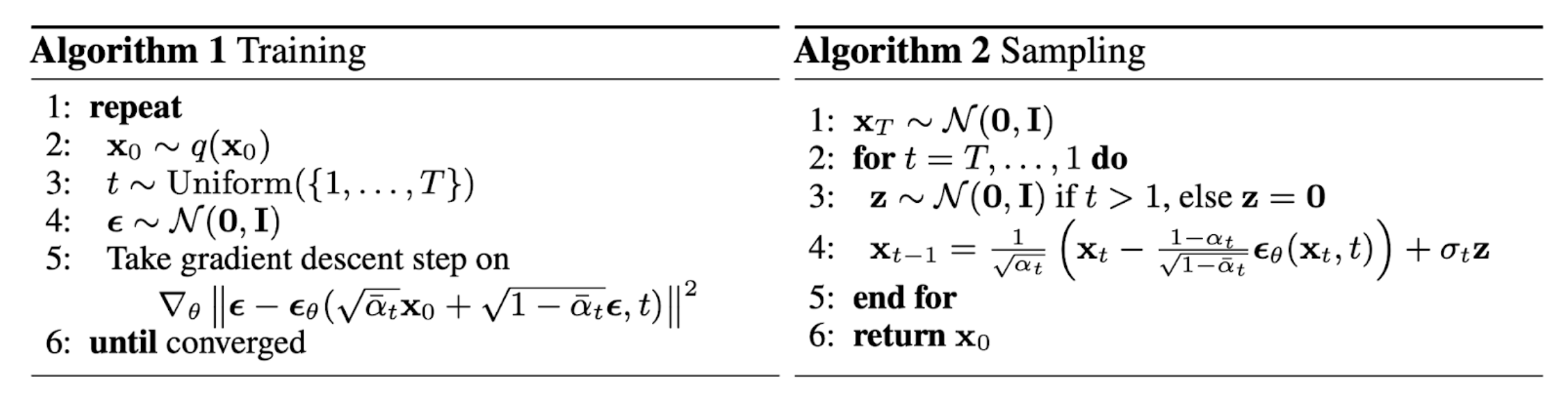
所以需要训练一个神经网络拟合这个概率分布,使用重参数化技巧,前向加噪声后,利用得到的图像数据得到高斯分布的参数μ

$$\begin{aligned} \boldsymbol{\mu}_{\theta}(\mathbf{x}_{t},t)& =\color{red}{\frac1{\sqrt{\alpha_t}}\left(\mathbf{x}_t-\frac{1-\alpha_t}{\sqrt{1-\bar{\alpha}_t}}\boldsymbol{\epsilon}_\theta(\mathbf{x}_t,t)\right)} \\ \Gamma\mathrm{hus~}\mathbf{x}_{t-1}& =\mathcal{N}(\mathbf{x}_{t-1};\frac{1}{\sqrt{\alpha_{t}}}\left(\mathbf{x}_{t}-\frac{1-\alpha_{t}}{\sqrt{1-\bar{\alpha}_{t}}}\boldsymbol{\epsilon}_{\theta}(\mathbf{x}_{t},t)\right),\boldsymbol{\Sigma}_{\theta}(\mathbf{x}_{t},t)) \end{aligned}$$ $$\begin{aligned} L_{t}& =\mathbb{E}_{\mathbf{x}_0,\epsilon}\Big[\frac{1}{2\|\boldsymbol{\Sigma}_\theta(\mathbf{x}_t,t)\|_2^2}\|\tilde{\boldsymbol{\mu}}_t(\mathbf{x}_t,\mathbf{x}_0)-\boldsymbol{\mu}_\theta(\mathbf{x}_t,t)\|^2\Big] \\ &=\mathbb{E}_{\mathbf{x}_0,\epsilon}\Big[\frac1{2\|\boldsymbol{\Sigma}_\theta\|_2^2}\|\color{red}{\frac1{\sqrt{\alpha_t}}\left(\mathbf{x}_t-\frac{1-\alpha_t}{\sqrt{1-\bar{\alpha}_t}}\boldsymbol{\epsilon}_t\right)}-\frac1{\sqrt{\alpha_t}}\Big(\mathbf{x}_t-\frac{1-\alpha_t}{\sqrt{1-\bar{\alpha}_t}} \\ &=\mathbb{E}_{\mathbf{x}_0,\boldsymbol{\epsilon}}\Big[\frac{(1-\alpha_t)^2}{2\alpha_t(1-\bar{\alpha}_t)\|\boldsymbol{\Sigma}_\theta\|_2^2}\|\boldsymbol{\epsilon}_t-\boldsymbol{\epsilon}_\theta(\mathbf{x}_t,t)\|^2\Big] \\ &=\mathbb{E}_{\mathbf{x}_0,\epsilon}\Big[\frac{(1-\alpha_t)^2}{2\alpha_t(1-\bar{\alpha}_t)\|\boldsymbol{\Sigma}_\theta\|_2^2}\|\boldsymbol{\epsilon}_t-\boldsymbol{\epsilon}_\theta(\sqrt{\bar{\alpha}_t}\mathbf{x}_0+\sqrt{1-\bar{\alpha}_t}\boldsymbol{\epsilon}_t,t)\|^2\Big] \end{aligned}$$

简化

$$\begin{aligned} L_{t}^{\operatorname{simple}}& =\mathbb{E}_{t\sim[1,T],\mathbf{x}_0,\boldsymbol{\epsilon}_t}\left[\|\boldsymbol{\epsilon}_t-\boldsymbol{\epsilon}_\theta(\mathbf{x}_t,t)\|^2\right] \\ &=\mathbb{E}_{t\sim[1,T],\mathbf{x}_0,\boldsymbol{\epsilon}_t}\left[\|\boldsymbol{\epsilon}_t-\boldsymbol{\epsilon}_\theta(\sqrt{\bar{\alpha}_t}\mathbf{x}_0+\sqrt{1-\bar{\alpha}_t}\boldsymbol{\epsilon}_t,t)\|^2\right] \end{aligned}$$

最终目标优化函数

$$L_\text{simple} = L_t^\text{simple} + C$$

加速扩散模型采样

DDPM生成样本很慢,可以通过经过多步后进行采样(也就是增加采样间隔),或者根据DDIM论文,跳过p(x~t~|x~t-1~)直接从p(x~t~|x~0~)出发.

$$\begin{aligned} \mathbf{X}_{t-1}& =\sqrt{\bar{\alpha}_{t-1}}\mathbf{x}_0+\sqrt{1-\bar{\alpha}_{t-1}}\boldsymbol{\epsilon}_{t-1} \\ &=\sqrt{\bar{\alpha}_{t-1}}\mathbf{x}_0+\sqrt{1-\bar{\alpha}_{t-1}-\sigma_t^2}\boldsymbol{\epsilon}_t+\sigma_t\boldsymbol{\epsilon} \\ &=\sqrt{\bar{\alpha}_{t-1}}\mathbf{x}_0+\sqrt{1-\bar{\alpha}_{t-1}-\sigma_t^2}\frac{\mathbf{x}_t-\sqrt{\bar{\alpha}_t}\mathbf{x}_0}{\sqrt{1-\bar{\alpha}_t}}+\sigma_t\boldsymbol{\epsilon} \\ q_\sigma(\mathbf{x}_{t-1}|\mathbf{x}_t,\mathbf{x}_0)& =\mathcal{N}(\mathbf{x}_{t-1};\sqrt{\bar{\alpha}_{t-1}}\mathbf{x}_{0}+\sqrt{1-\bar{\alpha}_{t-1}-\sigma_{t}^{2}}\frac{\mathbf{x}_{t}-\sqrt{\bar{\alpha}_{t}}\mathbf{x}_{0}}{\sqrt{1-\bar{\alpha}_{t}}},\sigma_{t}^{2}\mathbf{I}) \end{aligned}$$ $$\tilde{\beta}_t=\sigma_t^2=\frac{1-\bar{\alpha}_{t-1}}{1-\bar{\alpha}_t}\cdot\beta_t$$

参考资料

1. The Annotated Diffusion Model (huggingface.co)
2. diffusion_model.ipynb - Colaboratory (google.com)
3. cloneofsimo/minDiffusion: Self-contained, minimalistic implementation of diffusion models with Pytorch. (github.com)
4. What are Diffusion Models? | Lil’Log (lilianweng.github.io)
5. 生成扩散模型漫谈（一）：DDPM = 拆楼 + 建楼 - 科学空间|Scientific Spaces
6. Diffusion Models from Scratch in PyTorch (sungsoo.github.io)